Featured Posts (154)

Sort by
Subject:  Qfull in SWMM 5 for various levels of y/yFull in a Circular Pipe


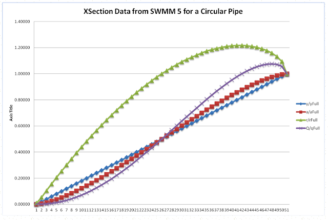
Here is a table that shows the value of Q/Qfull for various levels of y/yFull or d/D in SWMM5.  The full flow if you loop off the top of a circular pipe at the 0.83 level would be about 1.01 times Qfull for the whole pipe.  Figure 1 shows how the flows are calculated at various values, Table 1 and Figure 2 show the values of a/aFull, r/rFull and q/qFull for various values of y/yFull.


Figure 1.   How Qfull and Qmax are calculated in  SWMM 5 based on the roughness, slope and a lookup table for area and hydraulic radius for a circular pipe.


Image004


Table 1.   Table  of y/yFull and Q/Qfull based on a/aFull and r/rFull

y/yFull
a/aFull
r/rFull
Q/qFull
0.00000
0.00000
0.01000
0.00000
0.02000
0.00471
0.05280
0.00066
0.04000
0.01340
0.10480
0.00298
0.06000
0.02445
0.15560
0.00707
0.08000
0.03740
0.20520
0.01301
0.10000
0.05208
0.25400
0.02089
0.12000
0.06800
0.30160
0.03058
0.14000
0.08505
0.34840
0.04211
0.16000
0.10330
0.39440
0.05556
0.18000
0.12236
0.43880
0.07066
0.20000
0.14230
0.48240
0.08753
0.22000
0.16310
0.52480
0.10612
0.24000
0.18450
0.56640
0.12630
0.26000
0.20665
0.60640
0.14805
0.28000
0.22920
0.64560
0.17121
0.30000
0.25236
0.68360
0.19583
0.32000
0.27590
0.72040
0.22172
0.34000
0.29985
0.75640
0.24893
0.36000
0.32420
0.79120
0.27733
0.38000
0.34874
0.82440
0.30662
0.40000
0.37360
0.85680
0.33702
0.42000
0.39878
0.88800
0.36842
0.44000
0.42370
0.91760
0.40009

Figure 2.   Graph of values in Table 1
Read more…

Subject:   How is the Mass Balance Calculated in the SWMM 5 Groundwater Component?


The groundwater component of SWMM 5 is found in the gwater.c code.  It (as is all of SWMM 5) is excellently written in small functions by Lew Rossman of the EPA during the SWMM 5 development process.  However, code being code sometimes it is easier to see how the code is functioning.  This blog or note tries to show the mass balance local function updateMassBal


The groundwater component consists of groundwater data (gw in the equation) and aquifer data (a) in the equation.  The equation for the groundwater mass balance is shown in Figure 1.   The infiltration, evaporation occur only over the pervious area but the percolation out the bottom of the aquifer occurs over the whole Subcatchment.


Figure 1.  Groundwater Mass Balance


Image003 


Read more…

Subject:   How is the Volume Calculated in the SWMM 5 Groundwater Component?


The groundwater component of SWMM 5 is found in the gwater.c code.  It (as is all of SWMM 5) is excellently written in small functions by Lew Rossman of the EPA during the SWMM 5 development process.  However, code being code sometimes it is easier to see how the code is functioning.  This blog or note tries to show that function. 


The groundwater component consists of groundwater data (gw in the equation) and aquifer data (a) in the equation.  The equation for the groundwater volume is shown in Figure 1.   The volume is the water content (theta) times the upper depth and the porosity of the aquifer times the lower depth (Figure 2).


Figure 1.  Groundwater Volume Calculations


Image004


Figure 2.  Lower and Upper Depth of the Groundwater Compartrment


Image007


Read more…

Aquifer and Groundwater Objects in SWMM 5

Subject:   Aquifer and Groundwater Objects in SWMM 5


There are two types of data objects in SWMM 5 to describe the Groundwater flow component.  There is a Groundwater data object associated with a Subcatchment that describes flow equations, the interaction between the Subcatchment infiltration and the Groundwater component and an Aquifer data object that describes the characteristics of the Aquifer that may span one or more Subcatchments.  The Groundwater data is specific to one Subcatchment but the Aquifer may extend over more than one Subcatchment.


Image007

Image003


Read more…

Subject: Hierarchy of Your Network in InfoSWMM and H2OMAP SWMM

In both InfoSWMM and H2OMAP SWMM you can run a subset of the network by using the Facility Manager to make part of the network inactive and not solved.  You can make the output files smaller if you are performing a continuous simulation and save only the results of All, the Domain Only or a Selection Set to the graphical output file (Figure 1).   Figure 2 shows a few ways to query, view, graph and perform statistics for the model run.

Figure 1.  Options for saving the Active Network Data to the Graphical Output Data Set.

Figure 2.  Output View, Query and Graphical Options.

Read more…

Subject:  Advanced SWMM 5 import into InfoSWMM and H2OMAP SWMM

The current version of InfoSWMM and H2OMAP SWMM not only imports the latest SWMM 5 version but it has built in flexibility that allows the user to import selected data sections, model data sections or auxiliary file information such as calibration data files.  This allows you the choice of importing nonspecific network data that can used in the model of any city, county, shire, town or watershed.  For example,  you can import only these sections without affecting the geometry of your network:


1.      Calibration File Information,
2.      RTC Rules
3.      Aquifers
4.      Snowpacks
5.      Buildup for Water Quality,
6.      Washoff for Water Quality,
7.      Evaporation,
8.      Time Series,
9.       DWF,
10.        Patterns,
11.        RDII
12.        Loadings,
13.        Curves,
14.        LID Controls,
15.        LID Usage,
16.        Pollutants,
17.        Land Uses


Possible uses of this feature would be to have a city wide or companywide library of LID controls, RTC Rules or RDII values.


Figure 1.  Import Dialog with Import Options
Figure 2.  Only names and directories of the Calibration Files was imported


Subject:   Import of Sections from SWMM 5 into InfoSWMM and H2oMAP SWMM

A very useful hidden feature of the import SWMM 5 to InfoSWMM and H2OMAP SWMM is the ability to import all of the data or just one section.  For example, you can import the LID data, DWF patterns, control rules, pollutants, transects and other data that is transferable between different networks.

 
Read more…

Subject:   SWMM 5 Loss Term Values for various velocities and K values


SWMM 5 has three loss terms available for each link:  Entrance, Exit and Other losses.  The Entrance loss uses the upstream link velocity, the  Other loss uses the center link velocity and the Exit loss uses the downstream link velocity.  The general form of the loss term in the St. Venant equation is K*V^2/2g Table 1 shows the loss in feet of head for various combinations of velocity and K value.  If you want to  simulate a little loss of head at each node then a small value of K should be used otherwise the cumulative loss in the whole networks will be many feet of head.


  Loss Term units equals K * V^2/2g = ft/sec * ft/sec * sec^2/ft = ft


Table 1:  Loss in feet of head for various combinations of velocity and K values.


Velocity (ft/sec)

K

K

K

K

K

K

0.050

0.100

0.250

0.500

0.750

1.000

1

0.001

0.002

0.004

0.008

0.012

0.016

2

0.003

0.006

0.016

0.031

0.047

0.062

3

0.007

0.014

0.035

0.070

0.105

0.140

4

0.012

0.025

0.062

0.124

0.186

0.248

5

0.019

0.039

0.097

0.194

0.291

0.388

6

0.028

0.056

0.140

0.280

0.419

0.559

7

0.038

0.076

0.190

0.380

0.571

0.761

8

0.050

0.099

0.248

0.497

0.745

0.994

8

0.050

0.099

0.248

0.497

0.745

0.994

9

0.063

0.126

0.314

0.629

0.943

1.258

10

0.078

0.155

0.388

0.776

1.165

1.553


Read more…

SWMM 5 Inlet Control Culvert Equations

Subject:   SWMM 5 Inlet Control Culvert Equations


The newer option for SWMM 5 culverts uses three culvert classifications and associated equations to compute the inlet controlled flow into a culvert using the FHWA (1985) equations.  The culvert code in the culvert.c code of SWMM 5 uses:


1.   Two Equations for Unsubmerged culvert flow,

2.   One Equation for the Transition flow, and

3.   One Equation for Submerged flow.

Image005


Image002


Image003


Read more…

Subject:  SWMM 5 Culvert Data from FHWA, HDS No. 5, Hydraulic Design of Highway Culverts, 1985


If you use the culvert option in later versions of SWMM 5 then when the inlet control equation flow is less than the computed St Venant flow then the FHWA equations will be used for the current iteration in the SWMM 5 Dynamic Wave Solution.


Image002


culvert.pdf Download this file


Read more…

Subject:  Elevation Interpolation from a Contour in H2OMAP SWMM


The node invert elevation or the node maximum depth can be interpolated if you use the Elevation Interpolation Tool in H2OMAP SWMM.


Steps

Action

1.   Make a Contour Plot of the Node Invert Elevations.


Image005


2.   The Created Contours are now a layer in H2OMAP SWMM.


Image004


3.   Recreate the Invert Elevation from the Contour by using the Value Field and Interpolate Field.


Image006


4.   You can  also estimate the Maximum Depth of the Node from the Contour and the known Node Invert Elevation.


Image002


Read more…

Subject:  How to see what you have in the various scenarios of InfoSWMM


How to see what you have in the various scenarios – a tool I use a lot is Scenario Explorer which shows you how to see the various datasets associated with a data set along with the relationship between the Base and Various Child Scenarios.


Read more…

Variable Time Step in SWMM 5

 Variable Time Step in SWMM 5


v  The goal of the link lengthening in SWMM 5 it to meet the CFL time step condition for the full link depth and full link velocity at the chosen lengthening time step.  If the link does not meet the CFL condition then this means the time step needed is smaller than your selected lengthening time step.  SWMM 5 will make an hydraulically equivalent longer link with a smaller roughness but the same full flow velocity as the shorter link.


v  If you are running a simulation in which all of the pipes are exactly full – no surcharge in any pipe – and the variable time step then there would be no need for SWMM 5 to use anything other than the minimum of the routing or lengthening time step.  However, since most real networks have a mixture of partial flow, surcharged flow and pressure flow, the actual time step depth, velocity/Froude Number is different than the assumed full depth and full flow velocity.  For example, the depth can be higher at one end of the pipe and the velocity higher than full flow velocity due to the water surface slope being higher than the bed slope.  The only way SWMM 5 can now satisfy the CFL time step condition since the modified length is fixed is to lower the variable time step.


Read more…

Subject:   Reading the Output of Older SWMM 5 versions in Newer SWMM 5 Versions


It is very easy to read the output graphs and output text file from older versions of SWMM 5 in newer versions of SWMM 5 as long as the rules are followed:


1.   You need to have the RPT file for the InputFileName or InputFileName.RPT

2.   You need to have the OUT file for the InputFileName or InputFileName.OUT

3.   The File Size for InputFileName.RPT is greater than 0

4.   The Run Status for InputFileName.OUT is true based on the tests in CheckRunStatus

a.       // Starting from end of file, read byte offsets of file's sections

b.       // Read # time periods, error code & file signature

c.       // Read file signature & version number from start of file

d.       // Check if run was completed

e.       // Check if results were saved for 1 or more time periods

f.        // Check if correct version was used

g.       // Check if error messages were generated


Figure 1.   The RPT File or OUT File is not saved unless you 1st save the Current Simulation Results.

Image002


Figure 2.   The binary output file of SWMM 5.0.013 in SWMM 5.0.022

Image003

Read more…

All Possible Culverts Example Model in SWMM5

Note:  Attached is an example SWMM 5 model that has all 57 culvert types possible in SWMM 5 in one model.  The culverts are 57 small individual networks consisting of an inflow node, an upstream open channel, upstream node for the culvert, culvert link with culvert code, downstream node of the culvert, downstream open channel and finally an outfall node.  The culvert code and the shape of the culvert determine which FHWA equation is used to determine the flow INTO the Culvert during the simulation:

 1.   The flow from the St Venant Equation or

2.   The flow from the FHWA equation

 The minimum flow is used by the program. 


Image002


all_culverts.inp Download this file

Read more…

Note:   How Dry Weather Flow is Used in InfoSWMM at a Node


There are four components to the Dry Weather Flow (DWF) in InfoSWMM:


1.       The mean flow in user units at the node,

2.      The DWF Allocation Code – if you are using the DWF Allocator

3.      The Pattern for Weekday, Weekend etc for the mean flow.


The data is entered or entered for you in the Node Inflow Icon or the Operations Tab of the Attribute Browser


Node Inflow Icon and Associated Data

Image002


Operation Tab Patterns

Image003


You can also make global changes to your DWF using the Node DWF DB Table Under Extended Element Modeling Data

Image004


Image001

Read more…

Note:  SWMM5 Weir Rules and Head Calculations


This note attempts to explain both how the head upstream and the head downstream of a weir in SWMM 5 is calculated compared to the weir crest elevation and also to explain how the weir is presented in the HGL plot of SWMm 5.  There has been confusion in the past concering how the weir is shown compared to the actual weir calculations.  The node head is calculated obviously at both ends of the weir but the head over the weir is always based on H1-Crest or H2-Crest (Figure 1) and hence the weir should look flat – to the weir the downstream head is important but NOT the downstream node invert so the weir really is flat and should look flat in the HGL Profile across the weir (Figure 2).    The crest elevation is always relative to the upstream node invert elevation NOT the downstream node invert elevaation


Figure 1.  How the Head across a Weir is calculated in SWMM 5


Image005


Figure 2.   HGL Profile across a Weir in SWMM 5.0.022.  The black line should be shown flat.


Image003

Read more…

Time Step Approximation based on Link Lengths

Note:  A rough approximation of the time step you need for an InfoSWMM or H2OMAP SWMM model can be found by finding the mean link length using the field statistics tool for the length in the Conduit DB Table and then estimating the time step from the mean length, mean full depth velocity and mean full depth wave celerity.


The time step actually used during the simulation is related to this velocity and the safety adjustment factor.  The larger the safety adjustment factor the larger the mean time step listed in the Routing Time Step Suggestion.


Image002

Read more…

Subject - Smoother Switching Between Pumps in SWMM 5 - A better simulation of a VSP?


An oft requested feature in SWMM 5 is the ability to better simulate a variable speed pump.   The basic feature we are trying to model is multiple pumps between two nodes, one pump curve for all of the pumps and the ability to turn on and turn off the pumps based on either the head or depth at a Wet Well (Figure 1).  You can turn on or off the pumps Pump1, Pump2 and Pump3 based on the depth at the Wet Well but this feature is stepwise linear and usually uses three pump curves.  A better way to simulate this feature is to use the SWMM 5 Real Time Rules (RTC) to simulate the Pump setting based on a control curve.  


The Pump flow at any time step is the Pump Flow estimated from the Pump Curve (Figure 2) * The Pump Setting (Figure 3)


Each of the three pumps has a different Control Curve (Figure’s 4, 5 and 6, respectively) which turns on or turns off the Pump based on a range of Wet Well Depths.  The overall effect is that the total flow summing all three pumps together is smoother (Figure 7 and Figure 8) and the user can simulate different pump speeds based on the same pump curve depending on which pump is currently on.


Figure 1.   Example RTC Rules and VSP Pumps in a SWMM 5 model.


Image002

Figure 2.  The Pump Curve Used for all 3 Pumps


Image004


Figure 3.  The Pump Setting for all Three Pumps

Image003


Figure 4.   Pump Control Curve for Pump 1.  The Pump has a Setting of ¼ between 0.5 and 3 feet at the node Wet Well and zero otherwise.


Image005


Figure 5.   Pump Control Curve for Pump 2.  The Pump has a Setting of 1/2 between 3 and 5 feet at the node Wet Well and zero otherwise.

Image006


Figure 6.   Pump Control Curve for Pump 3.  The Pump has a Setting of 1 above 5 feet at the node Wet Well and zero otherwise.

Image007


Figure 7.  The Flow in all 3 Pumps.

Image008


Figure 8.  The total flow from all three Pumps to the downstream node.


Image009

Read more…