Pre 2014 Blogs

Subject:   How to Make a Smaller Model out of a Large Model in InfoSWMM

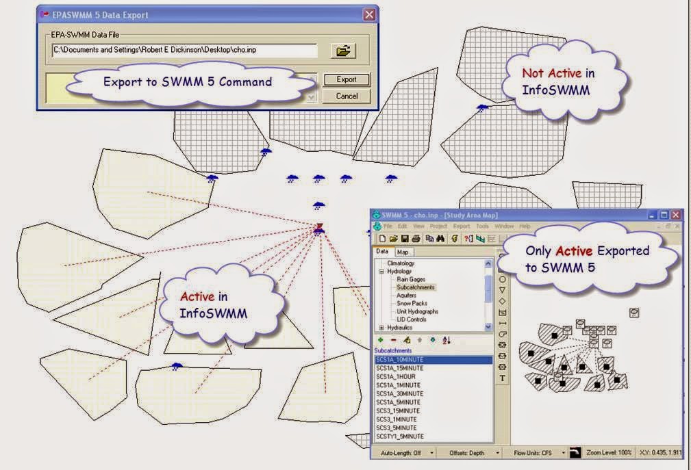
InfoSWMM and H2OMAP SWMM will export only those ACTIVE elements to SWMM 5 as defined by the Facility Manager. 

You can use the feature to make smaller SWMM 5 models and then reimport the exported smaller SWMM 5 model back into a H2OMAP SWMM or InfoSWMM scenario.

Subject:   The Importance of Viewing Results at the Proper Time Scale

 

In SWMM 5 when you are simulating rapidly changing flow – such as pump flows – it is important to  remember that you are only seeing the results of the simulation at your selected report time step.  Here is an example model with the same number of pump starts for all three simulations (318), the same  average time step during the simulation (10 seconds) but different report time steps.  The conception of the pump starts is totally different visually depending on the selected report time steps.  You should always compare the starts using the pump graphs and the pump summary table.    The percent utilized and the number of pump start ups tells you  the mean pump start length or in this case 153 seconds or 45.1 percent of 30 hours divided by 318 pump starts.

 

 

Subject:   An Example of the Importance of the Term DQ4 in the SWMM 5 St Venant Solution

The four terms are are used in the new flow for a time step of Qnew:

Thanks to Plants, We Will Never Find a Planet Like Earth

Earth's flora is responsible for the glaciers and rivers that have created this planet's distinctive landscape

Perhaps even more surprisingly, vascular plants formed the kinds of rivers we see around us today, according to another article by Martin Gibling of Dalhousie University in Nova Scotia and Neil Davies of the University of Ghent in Belgium, who analyzed sediment deposition going back hundreds of millions of years. Before the era of plants, water ran over Earth's landmasses in broad sheets, with no defined courses. Only when enough vegetation grew to break down rock into minerals and mud, and then hold that mud in place, did river banks form and begin to channel the water. The channeling led to periodic flooding that deposited sediment over broad areas, building up rich soil. The soil allowed trees to take root. Their woody debris fell into the rivers, creating logjams that rapidly created new channels and caused even more flooding, setting up a feedback loop that eventually supported forests and fertile plains.

 

"Sedimentary rocks, before plants, contained almost no mud," explains Gibling, a professor of Earth science at Dalhousie. "But after plants developed, the mud content increased dramatically. Muddy landscapes expanded greatly. A new kind of eco-space was created that wasn't there before."

Aging US water infrastructure has meant more leaks, flooded basements, and massive sinkholes in cities across the US. Fixing the water and sewer systems in need of repair will take billions of dollars, and it's hard to find that kind of money in the budget these days.

Saqib Rahim reports for ClimateWire on Philadelphia's decision to use "green infrastructure" rather than building a larger pipe system to handle the water that's dumped on the city during severe storms. The combination of more intense storms and more paved area is a problem: Impervious surfaces like roads, sidewalks, and parking lots can't absorb rainfall, so it ends up in the city's stormwater collection system -- which, in many older cities, is combined with the sewage system. When these combined systems are overwhelmed by heavy rainfall, the result is often that a rainfall-and-sewage mixture gets discharged into a local waterway. (Read more about this problem here.) Rahim explains Philadelphia's solution to this problem:

Instead of building an even larger pipe system to address the issue, [Water Department Commissioner Howard] Neukrug pitched the most aggressive "green infrastructure" plan in the country. Through increased vegetation, rain barrels, sponge-like roads and other measures, the city would try to absorb more water where it fell. The ground would filter out pollutants, reduce strain on the pipelines and make the city a more attractive place.

Neukrug tells Rahim that the green infrastructure solution will cost Philadelphia $2 billion, compared to $8 billion to $10 billion for larger underground tunnels. But the part of the city's plan that's currently causing a controversy is what water customers will pay. They'll now be charged not just for the water they use, but for their contributions to stormwater problems -- that is, sites with a lot of impervious surfaces will pay more.

The average household will see an average bill rise from approximately $60 to around $63.50, Rahim reports. For some large businesses, though, costs could rise significantly over the next few years -- and 100 of these businesses have hired a lobbyist and met with the Water Department to oppose implementation of the new billing practices.

I can understand why these businesses are upset. When they invest and plan for their businesses' futures, they assume the rules will stay the same. Their extensive impervious surfaces are causing problems for public health, but they might not have realized that their decisions about what to pave were raising costs for the city's residents (and everyone else affected when its sewage ended up in local waterways).

Changing the rules isn't ideal, but it's the best solution if the current rules create incentives for behavior that harms public health. If this country had never changed the rules to make businesses start bearing more of the cost for problems they cause the general public (externalities, in economic language), we'd still have rivers so polluted that they catch fire. Governments can ease the pain by providing grants or low-interest loans to help businesses and individuals invest in greener setups -- and, Rahim reports, Philadelphia is offering loans to businesses that want to green their facilities. Increases in bills will also be capped at 10% or $100 per month.

Such an approach could also be used to address other public health issues like CO2 emissions -- but so far, opposition to a carbon tax has been stronger than support. In the meantime, I'll be watching Philadelphia's effort and hoping it succeeds with a green solution to water infrastructure challenges.