Featured Posts (154)

Sort by

How to Model a Vacuum Sewer in SWMM 5


Subject:  How to Model a Vacuum Sewer in SWMM 5  


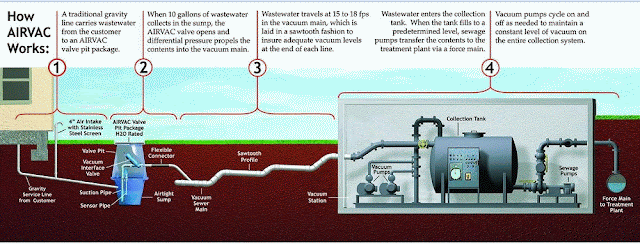
You can model a vacuum sewer as a gravity pipe connected to a storage node connected to an outlet connected to various pipes in a sawtooth pattern connected to a collection tank with a pump that pumps to a force main.

1.       Gravity Pipe,

2.       Storage Node,

3.       An Outlet function that works as a function of the depth in the storage node

4.       Series of Pipes in a Sawtooth Pattern,

5.       Collection tank,

6.       Pump

7.       Force Main

http://www.sivacvacuumsewer.com/index03.html
Vacuum Sewer Example
Read more…

SWMM 5 and InfoSWMM Time Step Guide

Subject:   SWMM 5 and InfoSWMM Time Step Guide

If you use a variable time step in SWMM 5 or InfoSWMM/H2OMAP SWMM it is hard to gauge the proper value of the conduit lengthening.  You want to use a value that does not increase the volume of the network yet does increase the length of the shortest links so you can use a longer time step.  A good approximation to the time step that you want to use is shown in the image.  


The Time Step Guide in seconds is Link Length / [Velocity + sqrt(g*Maximum Depth)] with the assumption that the velocity at maximum depth is about the value of the wave celerity for closed links or sqrt(g*Maximum Depth).  Normally (unless pumps are involved) the average time step used during the simulation is a good gauge of the time to use for the simulation.  For example, in this model run the time step used is 13 seconds which is about the conduit lengthening time step of 20 seconds * adjustment factor of 0.75 


Image002

Read more…

SWMM 5 Arrow Direction Question


Subject:   SWMM 5 Arrow Direction Question

question often asked is what happens to the flow in a SWMM 5 link if the downstream and upstream node names are entered in reverse.    The flow will be exactly the same as if the nodes were entered in the right order but the flow in the link will be negative.  As long as the inflow to the model is at the same node in both alternate models the node depth, the link upstream depths and upstream cross sectional areas will be the same.  For example, the flow out of Nodes 80408A and 80408 will be the same but the flow out of 80408 will be negative and the flow out of 80408A will be positive.


Read more…

Subject:  Siphon Simulation in SWMM 5 and InfoSWMM


A Siphon is simulated in SWMM 5 and InfoSWMM using the basic node and link data and downstream boundary condition:


1.   Inflow can be time series, dry weather flow pattern, wet weather inflow or Subcatchment Runoff,

2.   The boundary condition can be either a free outfall, fixed or time series,

3.   The node invert, node maximum depth and node surcharge depth are defined by the user or network,

4.   The link lengths, diameters, link offset depths upstream and downstream are defined by the user of the network,

5.   The node depths, link flows, link depths and link cross sectional areas are calculated at each time based on the node continuity equation and the link momentum and continuity equation.  The link flows are a function of the friction loss, head difference across the link and the difference in the cross sectional areas of the link.

6.   In the particular model the Inflow at node MH1 fills up the MH1 depth which causes the links downstream to start flowing – the head difference across the links drives the flow up and over the siphon.

Image002
Figure 1.  Example Siphon
Read more…

Subject:   3 Types of Subcatchment Flow in SWMM 5


There are three types of Subcatchment flow in SWMM 5 (Figure's 1 and 2)


1.   Impervious area with depression storage in which the runoff from the precipitation is delayed due to the depression storage.  Evaporation occurs based on the depth of water in the subarea of the Subcatchment.

2.   Impervious area without depression storage in which the runoff from precipitation is NOT delayed.  Evaporation does occur based on the depth of water in the subarea of the Subcatchment.

3.   Pervious area with depression storage in which the runoff from the precipitation is delayed due to the depression storage.  Evaporation and Infiltration occurs based on the depth of water in the subarea of the Subcatchment.


Image002
Figure 1.  Runoff from the 3 Types of Subcatchment Subareas


Image004
Figure 2: Subcatchment SubArea Types
Read more…

Subject:  SWMM 5 Clocktime RTC Rules for Pumps, Weirs and Orifices


You can use the Control or RTC rules in SWMM 5 to adjust the settings of the weirs, pumps and orifices based on the clock time each day of your simulation.  Here is an example that will adjust orifice height every ½ hour for 7 orifices at one time using two sets of rules.


RULE R1a 

; Half hour setting

IF SIMULATION CLOCKTIME = 0:30:00 

OR SIMULATION CLOCKTIME = 1:30:00  

OR SIMULATION CLOCKTIME = 2:30:00 

OR SIMULATION CLOCKTIME = 3:30:00 

OR SIMULATION CLOCKTIME = 4:30:00 

OR SIMULATION CLOCKTIME = 5:30:00 

OR SIMULATION CLOCKTIME = 6:30:00 

OR SIMULATION CLOCKTIME = 7:30:00 

OR SIMULATION CLOCKTIME = 8:30:00 

OR SIMULATION CLOCKTIME = 9:30:00 

OR SIMULATION CLOCKTIME = 10:30:00

OR SIMULATION CLOCKTIME = 11:30:00

OR SIMULATION CLOCKTIME = 12:30:00 

OR SIMULATION CLOCKTIME = 13:30:00  

OR SIMULATION CLOCKTIME = 14:30:00 

OR SIMULATION CLOCKTIME = 15:30:00 

OR SIMULATION CLOCKTIME = 16:30:00  

OR SIMULATION CLOCKTIME = 17:30:00 

OR SIMULATION CLOCKTIME = 18:30:00 

OR SIMULATION CLOCKTIME = 19:30:00 

OR SIMULATION CLOCKTIME = 20:30:00 

OR SIMULATION CLOCKTIME = 21:30:00 

OR SIMULATION CLOCKTIME = 22:30:00

OR SIMULATION CLOCKTIME = 23:30:00

THEN ORIFICE R1 SETTING = 0.90

AND  ORIFICE R2 SETTING = 0.90

AND  ORIFICE R3 SETTING = 0.90

AND  ORIFICE R4 SETTING = 0.90

AND  ORIFICE R5 SETTING = 0.90

AND  ORIFICE R6 SETTING = 0.90

AND  ORIFICE R7 SETTING = 0.90


RULE R1b

; hour setting

IF SIMULATION CLOCKTIME = 0:00:00

OR SIMULATION CLOCKTIME = 1:00:00

OR SIMULATION CLOCKTIME = 2:00:00

OR SIMULATION CLOCKTIME = 3:00:00

OR SIMULATION CLOCKTIME = 4:00:00

OR SIMULATION CLOCKTIME = 5:00:00

OR SIMULATION CLOCKTIME = 6:00:00

OR SIMULATION CLOCKTIME = 7:00:00

OR SIMULATION CLOCKTIME = 8:00:00

OR SIMULATION CLOCKTIME = 9:00:00

OR SIMULATION CLOCKTIME = 10:00:00

OR SIMULATION CLOCKTIME = 11:00:00

OR SIMULATION CLOCKTIME = 12:00:00 

OR SIMULATION CLOCKTIME = 13:00:00

OR SIMULATION CLOCKTIME = 14:00:00 

OR SIMULATION CLOCKTIME = 15:00:00

OR SIMULATION CLOCKTIME = 16:00:00

OR SIMULATION CLOCKTIME = 17:00:00

OR SIMULATION CLOCKTIME = 18:00:00 

OR SIMULATION CLOCKTIME = 19:00:00 

OR SIMULATION CLOCKTIME = 20:00:00 

OR SIMULATION CLOCKTIME = 21:00:00 

OR SIMULATION CLOCKTIME = 22:00:00 

OR SIMULATION CLOCKTIME = 23:00:00

THEN ORIFICE R1 SETTING = 0.5

AND  ORIFICE R2 SETTING = 0.5

AND  ORIFICE R3 SETTING = 0.5

AND  ORIFICE R4 SETTING = 0.5

AND  ORIFICE R5 SETTING = 0.5

AND  ORIFICE R6 SETTING = 0.5

AND  ORIFICE R7 SETTING = 0.5


Image002

Read more…

Subject:  Variables for Controlling the Continuity Error in InfoSWMM compared to SWMM 5


Time step is always a key parameter in SWMM 5 as it is the main parameter for a user to adjust in case of a significant continuity error.   InfoSWMM has additional flexibility and allows the user to control the number of Picard iterations and the Node continuity stopping tolerance.   SWMM 5.0.022 has the number of iterations fixed at 8 and the stopping tolerance fixed at 0.005 feet.   The stopping tolerance is important because it controls the number of iterations during a time step.  For example, if all of the Nodes have a current and former iteration depth difference (absolute) less than 0.005 feet then the time step is deemed converged and the node and link flow computations are stopped for that time step.  In SWMM 5 since the stopping tolerance is fixed then your main option is to reduce the time step.  In InfoSWMM you can also decrease the stopping tolerance, increase the number of iterations or decrease the time step.  In most models it is best to alter all three parameters for the fastest model.  For example, a slightly smaller maximum time step or a smaller variable time step adjustment factor, more iterations and a smaller tolerance will normally work better than just lowering the time step.


Image002


Read more…

Subject:   InfoSWMM 2D Layer Properties and Mesh Results


You can use the Layer Properties for layers in the Table of Contents to see the Mesh depth and other simulation data for the 2D mesh in InfoSWMM 2D.  The Mesh Depth can be seen using the Labels/Label Expression command and if you use an expression you can see the results data as well on the mesh.  The 2D depth on each Mesh can be viewed as either Pie or Bar Charts – the graph shown below is a small pie with the diameter of the pie a function of the depth.


Image003


Read more…

Subject:   InfoSWMM 2D Layer Properties and Mesh ID


You can use the Layer Properties for layers in the Table of Contents to see the Mesh ID and other simulation data for the 2D mesh in InfoSWMM 2D.  The Mesh ID can be seen using the Labels/Label Expression command and if you use an expression you can see the results data as well on the mesh.  The Mesh ID is used as the label as well in the 2D Output modeling report The Net Inflow and Net Outflow is by Mesh ID.  In this example, the flow comes out of Node 80408 to Mesh ID 131 and enters the 1D network again at Mesh ID 848.


Image002

Read more…

Subject:  SWMM 5 Fixed Surface Water Depth Boundary Condition


A large difference between SWMM 5 and SWMM 4 is how the Groundwater Aquifer interacts with the drainage network.  In SWMM 4 since the hydrology was simulated in the Runoff Block, the results saved to an interface file and the hydraulics were simulated in the Extran Block it was not possible to have a time step to time step interaction between the Aquifer and the Open Channels.  SWMM 5 has integrated hydrology and hydraulics so it is possible to use either a Fixed Surface Water Depth for each Subcatchment or the Receiving Nodes Node Depth Invert Elevation – the Aquifer Bottom Elevation.  The groundwater thus flows either to a fixed boundary condition as in SWMM 4 or to a time varying boundary condition.


Image003


Read more…

SWMM 5 Threshold Groundwater Elevation

Subject:  SWMM 5 Threshold Groundwater Elevation

A large difference between SWMM 5 and SWMM 4 is how the Groundwater Aquifer interacts with the drainage network.  InSWMM 4 since the hydrology was simulated in the Runoff Block, the results saved to an interface file and the hydraulics were simulated in the Extran Block it was not possible to have a time step to time step interaction between the Aquifer and the Open Channels.  SWMM 5 has integrated hydrology and hydraulics so it is possible to use either a fixed Threshold Groundwater Elevation for each Subcatchment or the Receiving Nodes Invert Elevation.


Read more…

Aquifers in SWMM 5

Subject:   Aquifers in SWMM 5


Groundwater in SWMM 5 is modeled as two zones: (1) Saturated and (2) Unstaturated.  The data for the Groundwater Simulation consists of physical data in an Aquifer and elevation and flow coefficient and exponent data in the Groundwater Data.  The Aquifer data object can be applied to multiple Subcatchments but each Subcatchment has its own set of Groundwater data.  For example, in this model all of the Subcatchments share the same Aquifer data but each Subcatchment has different elevation and flow data – the labels on the basin are the groundwater elevations. 


Image004

Read more…

Subject:  InfoSWMM and Arc GIS Layer Properties for Force Mains and Gravity Mains


An important advantage of using InfoSWMM is the ability to use all of the Arc GIS layer and programming tools.  For example, you can use the layer properties in the Table of Contents to color and create symbols for the force mains and gravity mains in InfoSWMM.  The Force Main variable (which is a Yes/No parameter) is selected as the field value in the Symbology Tab of Layer Properties which allows you to color and size the link based on the Force Main property of is you do a Layer Join the link property and simulation results.


Read more…

InfoSWMM Note About Pump Wet Wells

Subject:  Wet Well Maximum depths and Pump Start and Pump Off Depths
  The Wet Well has
·         An invert elevation and
·         A Maximum Depth
The Pumps have
·         Pump On Depth
·         Pump Off Depth
·         Pump Head – Discharge Curve or
·         RTC Rules
The Links have a
·         Invert Elevation into the Wet Well and
·         Invert Elevation into the Downstream Force Main
·         Crown Elevation
Figure 1. Wet Well  Maximum Depth
Read more…

Subject:  Detention Pond Infiltration and Evaporation Losses


You can also add a storage pond infiltration and surface evaporation losses to the pond.  The surface evaporation is added to the infiltration (computed from the green ampt parameters); a storage volume summary listing the average and maximum volume and the percent loss from the combined infiltration and evaporation from the ponds.  The pond infiltration loss during a time step is basd on the areal weighed average depth, the Green Ampt infiltration and the Area of the pond.


Image004
Figure 1.  Pond Infiltration Loss Assumptions


Image003
Figure 2. SWMM 5 Storage Summary listing Evaporation


Image002
Figure 3.  Infiltration Pond Data is entered in the Property Sheet for the Node.


infiltration_detetention_pond.inp Download this file

Read more…

Detention Basin Basics in SWMM 5

Subject:  Detention Basin Basics in SWMM 5


What are the basic elements of a detention pond in SWMM 5?  They are common in our backyards and cities and just require a few basic elements to model.  Here is a model in SWMM 5.0.022 that even has a fountain in the real pond – which we not model for now.   The components of the model are:


1.   An inlet to the pond with a simple time series – a subcatchment can be added to it in a more complicated model but for now we will just have a triangular time series,

2.   A pipe to simulate the flow into the pond from the inlet,

3.   Storage Node to simulate the Pond that consists of a tabular area curve to estimate the depth and area relationship,

4.   Storage Node to simulate the Outlet Box of the Pond

5.   Two Small Rectangular Orifices to simulate the low flow outflow from the pond at an elevation less than the weir

6.   A large rectangular orifice to simulate the normal inflow to the Box

7.   A rectangular weir to simulate the flow into the box when the pond water surface elevation is above the box

8.   The outlet of the Box is a circular link with a Free outfall as the downstream boundary condition

9.   The flow graph in the image shows the flow into the box starts from the two small orifices, next from the large orifice and finally from the top of the box or the weir.


Image002


2011-06-12_0826

detetention_pond.INP Download this file

Read more…

Subject:  Two new parameters and a modified table in InfoSWMM 11 and H2OMAP SWMM that does the following:


1.   Allows you to control the maximum number of iterations in the solution,

2.   Controls the Stopping tolerance (units of feet) for node iterations, and

3.   Shows not only the percent continuity error at a node but the error in million gallons (Mgal)


If you have a high continuity error or want to reduce your existing continuity error then you can increase the number of iterations or lower the stopping tolerance so that at each time step there is less continuity error. 


Image002

Read more…
Subject:  InfoSWMM Map Display of Scenario Differences

You can also make a table and map of the differences between the existing and future scenario.  The red in the image shows the pipes in which the flows have increased and the blue shows the pipes in which the flows have decreased between the existing and future scenarios.  You make the table by

1.       Making a conduit report for both scenarios at the same date/time,
2.      Copy the flow in the link for all links to Excel and make a new column with the difference between the future and existing conditions,
3.      Make a new column in the Conduit Information Table of InfoSWMM for real data and  paste the new column from Excel into the  Conduit Information Table,
4.      You then can use Map Display for links and show a Map Display of the flow differences at that particular date/time for all the links. 


Image002
Read more…


Every river system mapped in World of Rivers

March 28, 2011 to Mapping | Share on Twitter

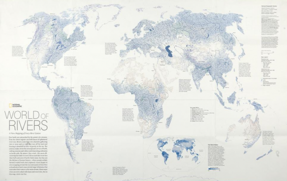
World of Rivers from NG

The annual Malofiej awards, for top graphics in journalism, were handed out last week. The best map of 2010 went to National Geographic for the World of Rivers. Every river system in the world was mapped and scaled by annual discharge.

We live on a planet covered by water, but more than 97 percent is salty, and nearly 2 percent is locked up in snow and ice. That leaves less than one percent to grow our crops, cool our power plants, and supply drinking and bathing water for households.

Showing everything doesn't always work with so much data, but it does in this case. It reminds me of Ben Fry's All Streets. See the full-sized interactive version on National Geographic.
 

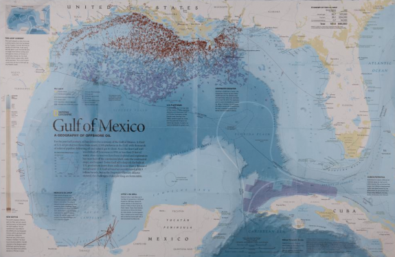
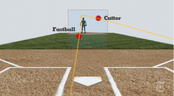
Also, congratulations to National Geographic for winning the Peter Sullivan award (best in show) for their map of the oil spill in the Gulf of Mexico and The New York Times for their work on how Mariano Rivera dominates, print and online, respectively.

[Society for News Design]

Via Flowing Data - http://flowingdata.com/2011/03/28/every-river-system-mapped-in-world-of-rivers/
Read more…