 |
|||||
|
|
|||||
|
Broomfield, Colorado USA, March 27, 2011 — MWH Soft is pleased to announce it has a new name, Innovyze. The new name and logo more accurately reflect the company’s rich history of creating innovative, technically advanced modeling and management solutions for the world’s water and wastewater communities.
“The name Innovyze brings together the best characteristics of innovation and analyze, which is represented in our combined organization. It means to introduce something new and to change, while carefully identifying key factors and possible results,” said Paul F. Boulos, Ph.D., Hon.D.WRE, F.ASCE, the company’s President and COO. “Although our name is changing, our people, products, and passion are still focused on our core mission: innovating for sustainable infrastructure.” As part of the introduction of the Innovyze name, the company has an updated website at www.innovyze.com and is hosting its first public event, the 2011 Asia Pacific Water and Sewer Systems Modelling Conference, beginning March 30 in Gold Coast, Australia. For additional information regarding the change, visit www.innovyze.com/newname. About Innovyze |
|||||
Featured Posts (154)
Sort by
Subject: Node Time Step in SWWM 5
The node time step in SWMM 5 is based on the maximum depth of the node, the last time step and the change in depth at the node between the current time step and the last time step. It is calculated at the beginning of each time step in the dynamic wave solution of SWMM 5. The maximum depth is the difference between the crown elevation of the node and the invert of the node. It is normally much less than the link time step in SWMM 5 and is only important at the beginning of the simulation when the depth between the current node depth and the old node is large (Figure 1). This is especially true if a hot start file is not used and the node starts out empty. If the node time step is smaller than the link time steps it will be listed in the Table Time Step Critical elements (Figure 2).
 |
| Figure 1. Equations for the Node Time Step. |
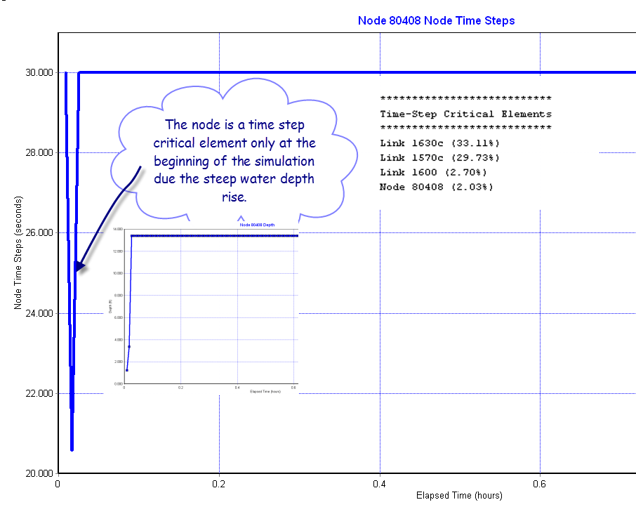 |
| Figure 2. Node Time Step is critical at the beginning of the simulation. |
|
MWH Soft Releases InfoSewer V7 with Significantly Enhanced
New release adds powerful analysis features for an improved modeling experience
|
||||||
|
Broomfield, Colorado USA, February 8, 2010 — MWH Soft, a leading global innovator of wet infrastructure modeling and simulation software and technologies, today announced the worldwide availability of the V7 Generation of InfoSewer for ArcGIS (Esri, Redlands, CA) platform. InfoSewer has helped define the standard in the industry for GIS-centric sanitary sewer network modeling and design since 2003. This seventh version of the software introduces key enhancements requested by customers that increase engineering productivity; improve network analysis and design; and enhance the visualization, comprehension, management and assessment of modeling results. Certified by the National Association of GIS-centric Software, InfoSewer is a powerful ArcGIS-centric software for use in planning, designing, analyzing, and expanding sanitary, storm and combined sewer collection systems. It can be effectively used to model both dry-weather and wet-weather flows and determine the most cost-effective and reliable method of wastewater collection. Built atop ArcGIS, InfoSewer enables engineers and GIS professionals to work simultaneously on the same integrated platform, commanding powerful geospatial analysis and hydraulic modeling in a single environment using a single dataset. InfoSewer is used worldwide by municipal engineers and planners to create detailed, accurate models of their sewer infrastructure systems. These models enable users to evaluate the effect of new developments, zoning changes, and other additional loads on system flows; pinpoint current and future problem areas; predict overflows and backups; and determine how to best restore needed capacity lost to infiltration and inflow with the least rehabilitation. In addition, users rely on these models to compute hydrogen sulfide generation and corrosion potential; analyze the rate of Biochemical Oxygen Demand (BOD) exertion; track sediment movement and deposition; trace pollutant contribution from source nodes, perform time of concentration pipe calculations; calculate the amount of pollutant transported to the wastewater treatment plant; and assess pollutants’ impacts on receiving waters. Extensive scenario management functionality enables the analysis of existing or future sewer collection systems. The application also provides vital tools for meeting and exceeding environmental regulations and improving community relations via database queries and map displays. The new InfoSewer V7 delivers advanced design functionality and exponential increases in efficiency while simplifying use, and improves speed and reliability by using memory more efficiently when working with large models. In addition to refinements throughout, users can now quickly and reliably design new sewer collection systems that consider standard design criteria such as flow depth-to-pipe diameter ratios, velocity, slope, soil cover depth, and pipe crown drop. Using user-input manhole locations and rules, InfoSewer V7 calculates the optimal pipe and slope, invert elevation of conduits and manholes, soil cover depths at both ends of each pipe section, and cost of excavation and reinstatement to meet target design criteria. Results can be reviewed using profile plots with advanced labeling of 30 node and link variables, color coded sewer maps of these variables, or 20 comprehensive tabular reports. The profile plots can be automatically updated in the model database for steady state and extended period simulations of new and existing designs, greatly simplifying the model building process. Together, these important modeling capabilities will help wastewater utilities worldwide dramatically raise productivity and efficiency by rapidly developing practical and optimal capital improvement strategies that minimize costs while improving system reliability, integrity and performance. By making engineering professionals more productive and their organizations more competitive, InfoSewer V7 delivers benefits utilities can pass on to their customers through better designs and higher quality standards, achieved in a shorter turnaround time. |
Note: How to Calculate the Freeboard of a Node in InfoSWMM/H2OMAP SWMM from the Model Results
The freeboard for a node in InfoSWMM/H2OMAP SWMM can be calculated with a 4 step process:
1. Copy the Node Rim Elevations from the DB Tables for Junctions to Excel,
2. Run the model and then copy the Maximum HGL from the Junction Summary output table to Excel,
3. Calculate the Freeboard in Excel as the Rim Elevation minus the Maximum HGL in Excel,
4. Create a new column called Freeboard in the Junction Information DB Table and paste the Freeboard from Excel.
You will be able to perform Map Displays or Map Queries now using the new Freeboard information column.
 |
| Figure 1. 4 Step Process to Calculate Freeboard |
Subject: What are the Units for the five St. Venant Flow Terms in SWMM 5 and InfoSWMM?
This is how the flow is calculated in a link in SWMM5. It uses the
· Upstream and downstream head,
· The user input length,
· The weighted cross sectional area and hydraulic radius as I explained in the previous email,
· The Center velocity,
· The Center Cross sectional area, and
· The Upstream and Downstream Cross sectional area.
The slope as listed in the output file is more for reference and is actually not used in the St. Venant Solution. The way the program usually works is that the friction slope lags the water surface head slope with the difference made up by the change in flow. The two non linear terms are usually small and only affect the flow during reverse or backwater events.
The new flow (Q) calculated at during each iteration of time step as
(1)Q for the new iteration = (Q at the Old Time Step – DQ2 + DQ3 + DQ4 ) / ( 1.0 + DQ1 + DQ5)
In which DQ2, DQ3 and DQ4 all have units of flow (note internally SWMM 5 has units of CFS and the flows are converted to the user units in the output file, graphs and tables of SWMM 5).
The equations and units for DQ2, DQ3 and DQ4 are:
(2)Units of DQ2 = DT * GRAVITY * aWtd * ( H2 – H1) / Length = second * feet/second^2 * feet^2 * feet / feet = feet^3/second = CFS
(3)Units of DQ3 = 2 * Velocity * ( aMid – aOld) * Sigma = feet/second * feet^2 = feet^3/second = CFS
(4)Units of DQ4 = DT * Velocity * Velocity * ( aDownstream – aUpstream) * Sigma / Length = second * feet/second * feet/second * feet^2 / feet = feet^3/second = CFS
The equations and units for DQ1 and DQ5 are:
(5)Units of DQ1 = DT * GRAVITY * (n/PHI)^2 * Velocity / Hydraulic Radius^1.333 = second * feet/second^2 * second^2 * feet^1/3 * feet/second / feet^1.33 = Dimensionless
(6)Units of DQ5 = K * Q / Area / 2 / Length * DT = feet^3/second * 1/feet^2 * 1/feet * second = Dimensionless
The five components calculated at the each time step and at each iteration during a time step and together predict the new Link Flow (Q) in SWMM 5. The value of the different components can be seen over time in Figure 1 and as a component percentage in Figure 2 and 3.

Figure 1: The Five St. Venant Components over time.

Figure 2: The relative magnitude of the St Venant terms over time for the same for the same link as in Figure 1.

Figure 3: The relative magnitude of the St Venant terms over time for the same for the same link as in Figure 1 shown in an area chart normalized to 100 percent. Normally the DQ1 and DQ2 terms balance each other except for backwater conditions or reverse flow in which the terms DQ3 and DQ4 can dominate.
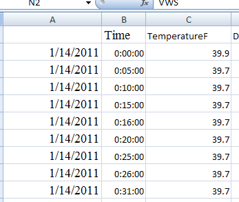
Subject: Weather Underground Temperature Data and SWMM 5
Weather Underground is a site that provides excellent local weather information in the form of graphs, tables and csv files. You can use the data very easily in SWMM 5 by copying from Excel to a time series in SWMM 5 and then use either the wind speed, precipitation or temperature in a model.
|
|
|
|
|
Figure 1. Weather Underground Temperature Data |


Figure 2. Save the Data to Excel by using the Comma Delimited File Command.
|
|
|
Figure 3. CSV File Exported to Excel |
|
|
|
Figure 4: Make a SWMM 5 Time Series to Copy and Paste the Temperature from the CSV File. |

The data imported from the csv file to Excel and after the text to columns tool is used looks like this in Excel. The data is now ready to be imported into SWMM 5 as is by copying and pasting from Excel to a SWMM 5 time series file. You need to perform the following steps:
1. Make a new SWMM 5 Time Series,
2. Copy and Paste the Temperature data from Excel to the SWMM 5 Time Series,
3. Use the Climatelogy Data Tab and select the new Temperature Time Series as the source of the simulation temperature,
4. You can see the simulated temperature by graphing the System Temperature.
|
|
|
Figure 5. SWMM 5 Climatology Tab and the resultant System Variable Graph of the Temperature. |

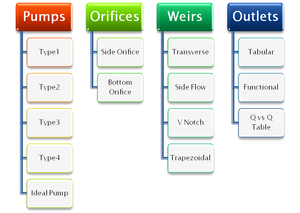
Subject: Diversion Links in SWMM 5 and 5.0.021
Diversion links in SWMM 5 are Pumps (5 types), Orifices (2 types), Weirs (4 types) and Outlets (3 types).
|
|
|
Figure 1. Diversion Links in SWMM 5 |
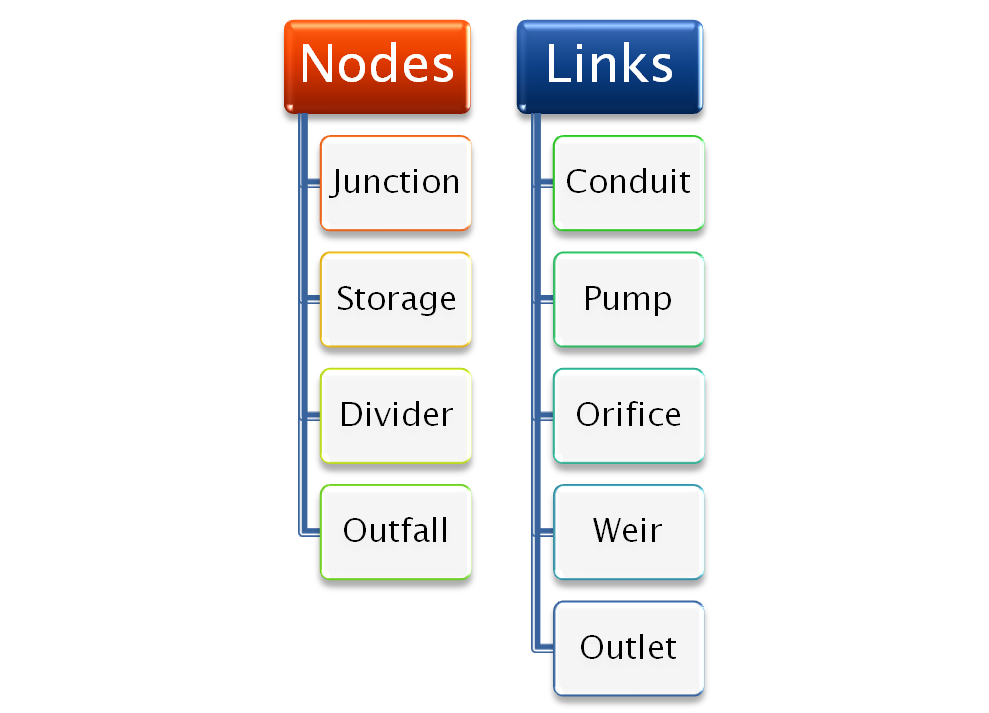
Subject: Types of Nodes and Links in SWMM 5
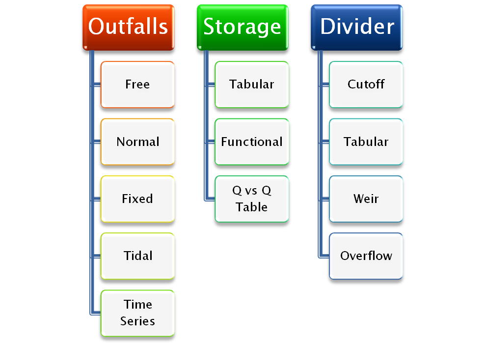
The main objects in a SWMM 5 drainage network are the nodes and links. Nodes are Junctions, Storages, Dividers and Outfalls. Links are Conduits, Pumps, Orifices, Weirs and Outlets. There is one type of junction but 5 types of Oufalls, 3 types of Storages and 4 types of Dividers. The dividers can be used in the dynamic wave solution of SWMM 5 but only divide the flow in the kinematic wave solution.
|
|
|
Figure 1. Node and Link Objects in SWMM 5 |
|
|
|
Figure 2: Node Objects in SWMM 5 |
Subject: SWMM 5 will iterate for the new node depth at each time for a minimum of 2 iterations to a maximum of 8 iterations based on the Node Continuity equation. If you plot the average number of iterations over time then typically the number of iterations go up as the Inflow increases. The nodes with the most iterations changes over time as the peak flow moves through the network as shown in this plan view. The iterations used during the simulation is a function of the node stop tolerance which has a default value of 0.005 feet in SWMM 5.


Note: Tributary Area to a Node in InfoSWMM
Here are the steps you neeed to take to calculate the tributary area of a node in InfoSWMM:
Step 1: Use the DB Editor to get the total area in your model using the Data Statistics Tool.

Step 2: Use the Process options in InfoSWMM to ONLY simulate surface runoff and flow routing.

Step 3. Copy the Node name and Total Inflow Volume from the Juntion Summary Output Table to Excel

Step 4: Find the Total Wet Weather Flow during the simulation from the Wet Weather Inflow Row in the Flow Continuity Table.
Dry Weather Inflow 0.000 0.000
Wet Weather Inflow 0.782 0.255
Step 5. Make a new column in Excel to calculate the tributary area.
The Tributary Area of a Node = Total Inflow Volume / Total Wet Weather Flow * Total Subcatchment Area from Step 1.
You will now have the tributary area for each node. You can verify this number = the total tributary area at the outfalls should equal the Total Subcatchment Area from Step 1.
|
Maximum |
Maximum |
|||||||
|
Lateral |
Total |
Time |
of |
Lateral |
Total |
Tributary |
||
|
Inflow |
Inflow |
Occurrence |
Volume |
Inflow |
Inflow |
Area |
||
|
Node |
Type |
CFS |
CFS |
days |
hr:min |
10^6 gal |
10^6 gal |
acres |
|
P001 |
JUNCTION |
5.54 |
10.86 |
0 |
2:27 |
0.1 |
0.255 |
14.74 |
|
P005 |
JUNCTION |
2.14 |
7.42 |
0 |
2:26 |
0.039 |
0.155 |
8.96 |
|
P009 |
JUNCTION |
5.78 |
5.78 |
0 |
2:25 |
0.106 |
0.106 |
6.13 |
|
P011 |
JUNCTION |
0.7 |
0.7 |
0 |
2:34 |
0.01 |
0.01 |
0.58 |
|
OUTLET |
OUTFALL |
0 |
10.84 |
0 |
2:28 |
0 |
0.255 |
14.74 |
Subject: Rain Barrel LID Summary


Subject: Rain Barrel LID Fluxes in SWMM 5.0.021
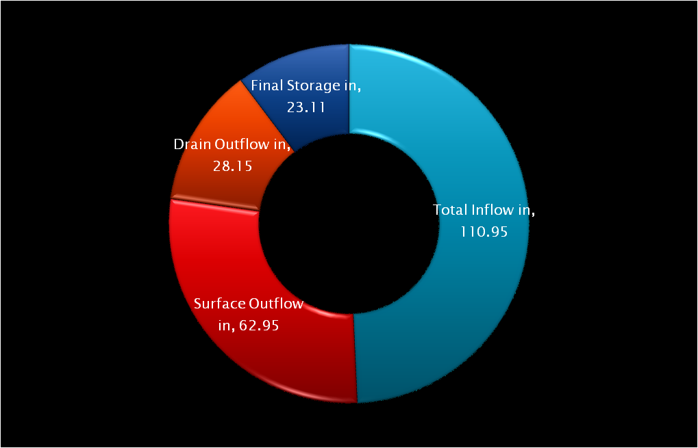
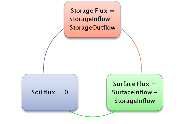
The fluxes are limited in a Rain Barrel Low Impact Development (LID) control in SWMM 5. The fluxes only include (Figure 1 and Figure 2):
1. Total Inflow,
2. Surface Outflow,
3. Drain Outflow and
4. Final Storage
The fluxes are also listed in the LID Performance Summary Table in the output text file.
***********************
LID Performance Summary
***********************
----------------------------------------------------------------------------------------------------------
Total Evap Infil Surface Drain Init. Final Pcnt.
Inflow Loss Loss Outflow Outflow Storage Storage Error
Subcatchment LID Control in in in in in in in
-----------------------------------------------------------------------------------------------------------
S1 RainBarrels 110.95 0.00 0.00 62.95 28.15 0.00 23.11 -2.94
 |
| Figure 1. Flux Pathways for a Rain Barrel LID |
 |
| Figure 2. Rain Barrel LID Fluxes |
Subject: Rain Barrel LID Drain Outflow in SWMM 5.0.021
The drain outflow in a Rain Barrel LID is defined by the user defined drain coefficient and drain exponent and the simulation storage depth The storage outflow does not occur until it has been dry for at least the drain delay time in hours.
The drain outflow in a Rain Barrel LID is defined by the user defined drain coefficient and drain exponent and the simulation storage depth The storage outflow does not occur until it has been dry for at least the drain delay time in hours.
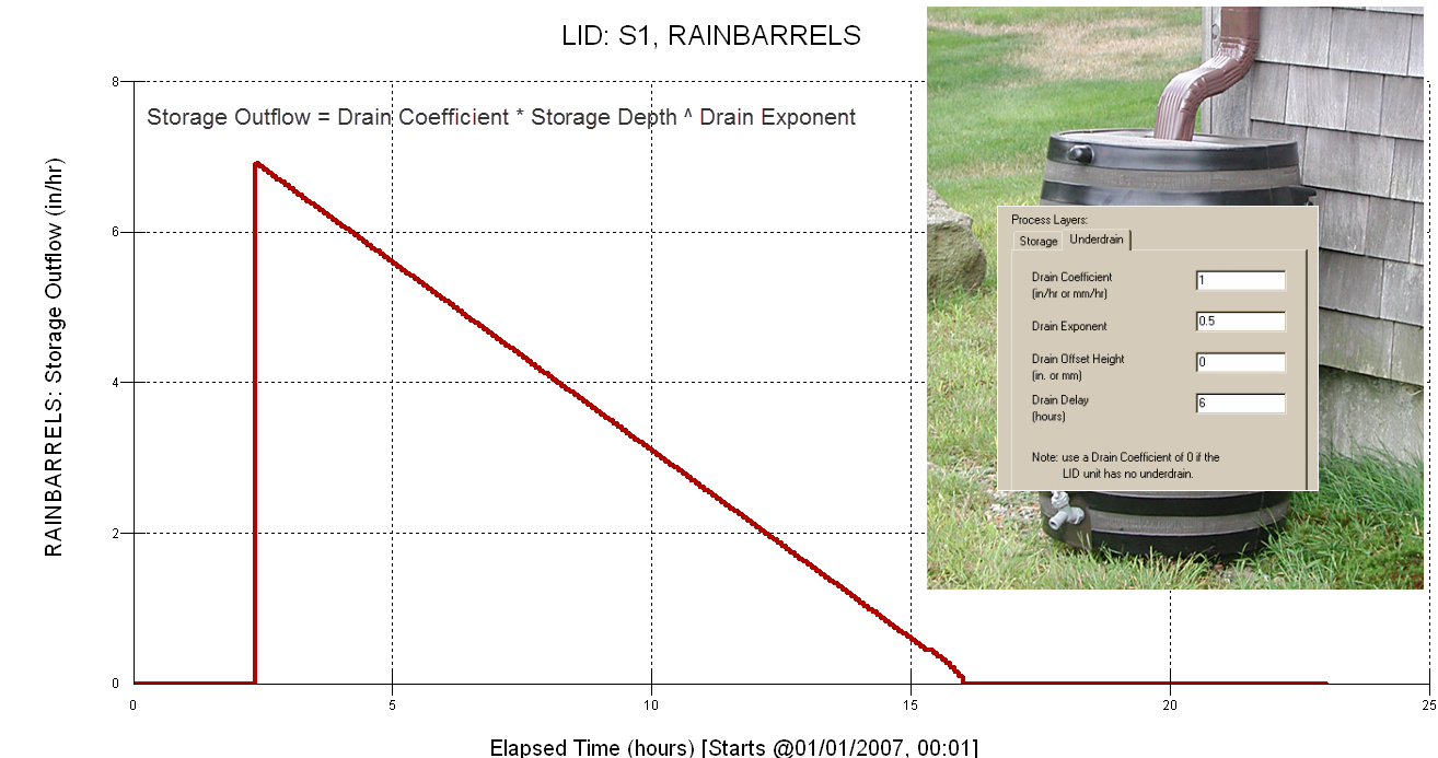 |
| Figure 1. Storage Outflow or Drain Outflow for a Rain Barrel LID |
 |
| Figure 2. You can see the effect of the Drain Delay in the output file for LID Simulation. |
Subject: Rain Barrel LID Storage Depth in SWMM 5.0.021
The storage depth in a Rain Barrel LID is limited by the user defined maximum rain barrel height in inches or millimeters. A rain barrel is one of the new LID features in SWMM 5.0.021
The storage depth in a Rain Barrel LID is limited by the user defined maximum rain barrel height in inches or millimeters. A rain barrel is one of the new LID features in SWMM 5.0.021
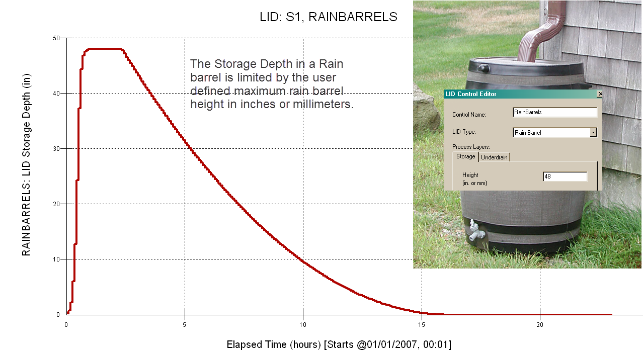 |
| Figure 1. Storage Depth in a Rain Barrel LID |
Subject: Link and Node Basics in SWMM 5 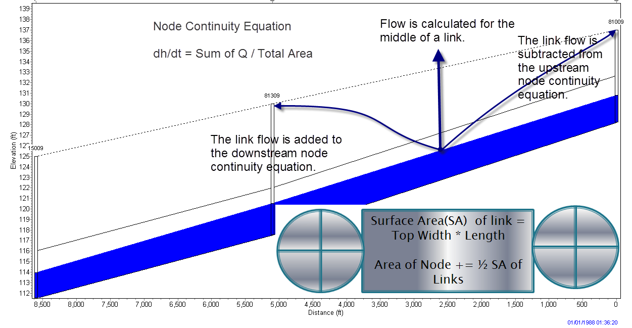
|
Figure 1. Link and Node Basics in SWMM 5 |
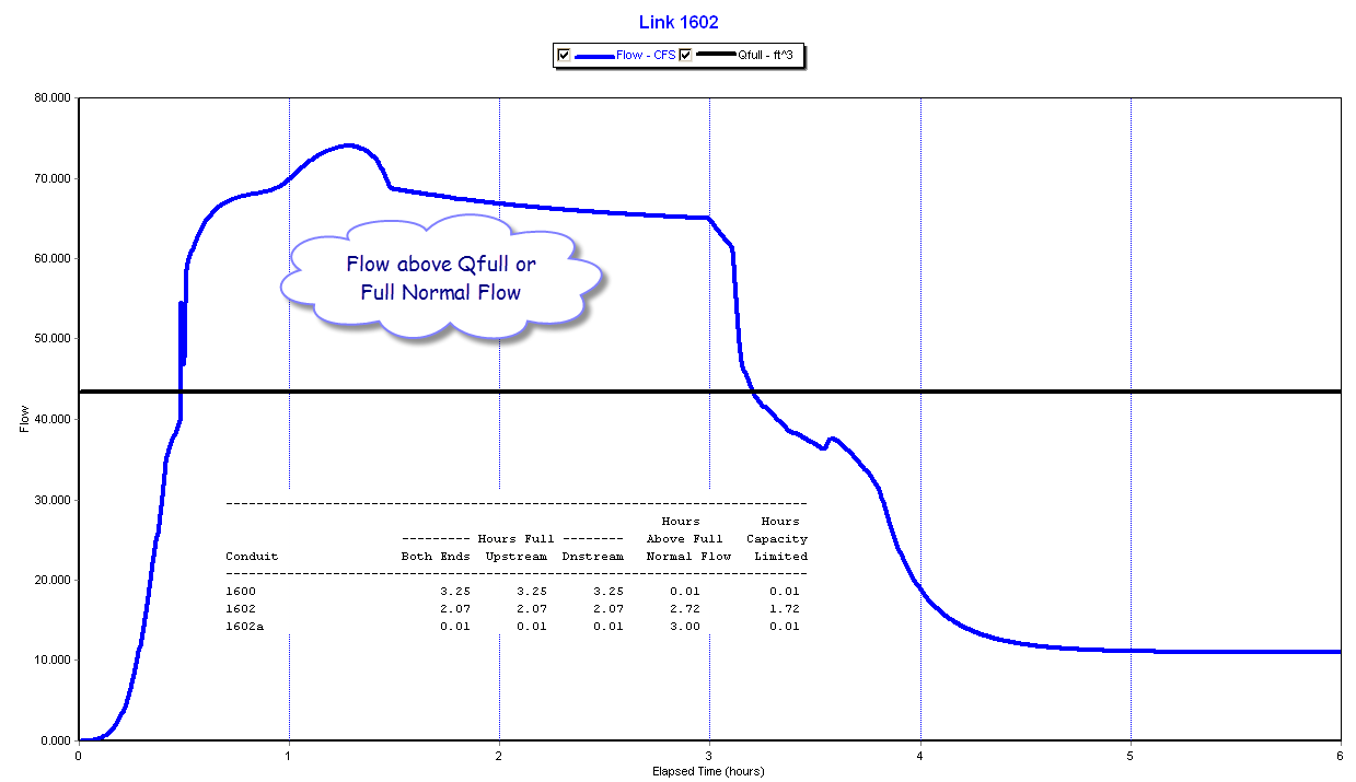
Subject: What is Hours Above Full Normal Flow in SWMM 5?
The Conduit Surcharge Summary Table in the Report text file or Status Report lists a column of results called “Hours above Full Normal Flow”. This is the number of hours the flow in the link was above the REFERENCE full flow as calculated by Manning’s equation. The flow in the link can be above full flow even if the link is not a full depth if the head difference across the link is high enough. The head difference is the water surface elevation at the upstream end of the link minus the water surface elevation at the downstream end of the link. The capacity or d/D of the link varies from 0 to 1 with 1 being a full pipe or link.
|
|
|
Figure 1. Hours above Normal Flow in SWMM 5 Links |
|
|
|
Figure 2. Flow versus Full Flow in SWMM 5 |

Subject: Area Types in SWMM 5 for Links with Offsets
There are six types of link flow in SWMM 5:
1. Dry Conduit at both Ends
2. Upstream End is Dry
3. Downstream End is Dry
4. Subcritical Flow
5. SuperCritical Flow
6. Free Fall at Upstream End
7. Free Fall at Downstream End
There are six types of link flow in SWMM 5:
1. Dry Conduit at both Ends
2. Upstream End is Dry
3. Downstream End is Dry
4. Subcritical Flow
5. SuperCritical Flow
6. Free Fall at Upstream End
7. Free Fall at Downstream End
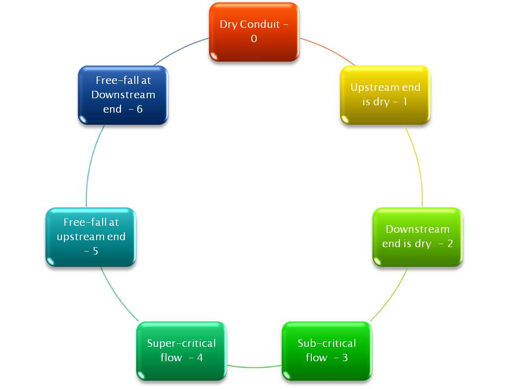 |
| Figure 1. Six types of Link Area Allocation |
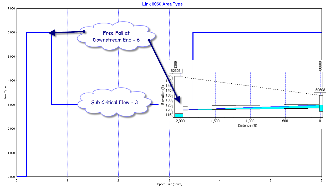 |
| Figure 2. Example Link Area Type in SWMM 5 |
Subject: Force Main Friction Loss in SWMM 5
You can model Force Mains in SWMM 5 using either Darcy Weisbach or Hazen Williams as the full pipe friction loss method (see Figure 1 for the internal defintion of full flow). No matter which method you use for full flow the program will use Manning’s equation to calculate the loss in the link when the link is not full (see Figure 2 for the equations used for calculating the friction loss – variable dq1 in SWMM 5). The regions for the different friction loss equations are shown in Figure 3.
You can model Force Mains in SWMM 5 using either Darcy Weisbach or Hazen Williams as the full pipe friction loss method (see Figure 1 for the internal defintion of full flow). No matter which method you use for full flow the program will use Manning’s equation to calculate the loss in the link when the link is not full (see Figure 2 for the equations used for calculating the friction loss – variable dq1 in SWMM 5). The regions for the different friction loss equations are shown in Figure 3.
 |
| Figure 1. How the full pipe condition is defined in SWMM 5 |
 |
||
Figure 2: Friction equations used in SWMM 5 for a Force Main.
|

Subject: Capacity Limited Links in SWMM 5
The table in the text report file of SWMM 5 called “Conduit Surcharge Summary” has a column entitled “Hours Capacity Limited” Here is how a link is defined as Capacity Limited in SWMM 5. Two factors have to be present:
1. The upstream end of the link has to be full and
2. The HGL Slope has to be greater than the Slope of the Link
Subject: What is the Area of a Node in SWMM 5?
The minimum area of a node is the default area of the node, which is the user defined minimum surface area or 12.566 square feet if the user does not define the surface area of the node. The surface area of a node is usually the half of the surface area of all of the connecting conduits but if the link is dry then the sum of all of the surface areas may be less than the default surface area. If you look at a scatter plot of the area versus the depth then you will see that it always has the minimum surface area.