All Posts (522)

Sort by

Emulation, Simulation, and the Human Brain

Emulation, Simulation, and the Human Brain

On this week’s episode of the EconTalk podcast, Russ Roberts asked Robin Hanson on the show to discuss his theory of the technological singularity. In a nutshell, Hanson believes that in the next few decades, humans will develop the technologies necessary to scan and “port” the human brain to computer hardware, creating a world in which you can create a new simulated copy of yourself for the cost of a new computer. He argues, plausibly, that if this were to occur it would have massive effects on the world economy, dramatically increasing economic growth rates.

But the prediction isn’t remotely plausible. There’s no reason to think it will ever be possible to scan the human brain and create a functionally equivalent copy in software. Hanson is confused by the ease with which this sort of thing can be done with digital computers. He fails to grasp that the emulation of one computer by another is only possible because digital computers are the products of human designs, and are therefore inherently easier to emulate than natural systems.

First a quick note on terminology. Hanson talks about “porting” the human brain, but he’s not using the term correctly. Porting is the process of taking software designed for one platform (say Windows) and modifying it to work with another (say Mac OS X). You can only port software you understand in some detail. The word Hanson is looking for isemulation. That’s the process of creating a “virtual machine” running inside another (usually physical) machine. There are, for example, popular video game emulators that allow you to play old console games on your new computer. The word “port” doesn’t make any sense in this context because the human brain isn’t software and he’s not proposing to modify it. What he means is that we’d emulate the human brain on a digital computer.

But that doesn’t really work either. Emulation works because of a peculiar characteristic of digital computers: they were built by a human being based on a top-down specification that explicitly defines which details of their operation are important. The spec says exactly which aspects of the machine must be emulated and which aspects may be safely ignored. This matters because we don’t have anywhere close to enough hardware to model the physical characteristics of digital machines in detail. Rather, emulation involves re-implementing the mathematical model on which the original hardware was based. Because this model is mathematically precise, the original device can be perfectly replicated.

You can’t emulate a natural system because natural systems don’t have designers, and therefore weren’t built to conform to any particular mathematical model. Modeling natural systems is much more difficult—indeed, so difficult that we use a different word, “simulation” to describe the process. Creating a simulation of a natural system inherently means means making judgment calls about which aspects of a physical system are the most important. And because there’s no underlying blueprint, these guesses are never perfect: it will always be necessary to leave out some details that affect the behavior of the overall system, which means that simulations are never more than approximately right. Weather simulations, for example, are never going to be able to predict precisely where each raindrop will fall, they only predict general large-scale trends, and only for a limited period of time. This is different than an emulator, which (if implemented well) can be expected to behave exactly like the system it is emulating, for as long as you care to run it.

Hanson’s fundamental mistake is to treat the brain like a human-designed system we could conceivably reverse-engineer rather than a natural system we can only simulate. We may have relatively good models for the operation of nerves, but these models are simplifications, and therefore they will differ in subtle ways from the operation of actual nerves. And these subtle micro-level inaccuracies will snowball into large-scale errors when we try to simulate an entire brain, in precisely the same way that small micro-level imperfections in weather models accumulate to make accurate long-range forecasting inaccurate.

Scientists have been trying to simulate the weather for decades, but the vast improvements in computing power in recent decades have produced only modest improvements in our ability to predict the weather. This is because the natural world is much, much more complex than even our most powerful computers. The same is true of our brains. The brain has approximately 100 billion neurons. If each neuron were some kind of simple mathematical construct (in the sense that transistors can be modeled aslogic gates) we could imagine computers powerful enough to simulate the brain within a decade or two. But each neuron is itself a complex biological system. I see no reason to think we’ll ever be able to reduce it to a mathematically tractable model. I have no doubt we’ll learn a lot from running computer simulations of neurons in the coming decades. But I see no reason to think these simulations will ever be accurate (or computationally efficient) enough to serve as the building blocks for full-brain emulation.

Read more…

2010 Was The Hottest and Wettest Year Ever

2010 Was The Hottest Year Ever 

Don’t look now, but climate change is still real:


The National Oceanic and Atmospheric Administration (NOAA) today announced that “2010 tied with 2005 as the warmest year of the global surface temperature record,” and 2010 is also “the wettest year on record, in terms of global average precipitation.” The year was by far the hottest during a La Niña cycle, during which the equatorial Pacific Ocean is unusually cold.

I seem to recall George Will and others getting very excited when 2006, 2007, 2008, and 2009 were all slightly cooler than 2005 since somehow that proved there was no warming trend. Oh well.

Read more…

Lightning


cbair.jpg

Source: http://florica.wordpress.com/2008/02/23/lightning/

Lightning is an electrical discharge, it can occur during thunderstorms, volcanic eruptions, nuclear reactions, forest fires where the dust creates a static charge or it can be triggered in a lab. Lightning is the sudden release of built-up charge stored in an electric field, though exactly what triggers it remains a mystery. There are many different types of lightning:

* cloud-to-ground, this is the archetypal lightning bolt, one that arcs out of the sky and strikes the ground with a flash of light.

lightning1.jpg

* cloud discharge, this is lightning that occurs within a thundercloud, between two thunderclouds, or from a thundercloud to the air. Cloud discharges are certainly more common than the cloud-to-ground variety: 10 or more cloud flashes may occur before the first one that strikes the earth.

02-vari-cloudtocloud.jpg

* ball lightning, there are not many scientific documentations such as videos, or other recordings of ball lightning, so experts have had to rely on eyewitness accounts, which have been numerous. Judging from such accounts, balls of lightning are typically between a golfball and a basketball in size, about as bright as a 60-watt light bulb, and often red, orange, or yellow in color. Observed shooting through the air, across the ground, and or even into houses, they are fleeting, generally lasting a few seconds before vanishing gradually or abruptly.

403487aa2.jpg

*blue jet, blue jets shoot upward from the tops of thunderclouds. This remoteness, and the fact that they last but a few hundred milliseconds at most, perhaps accounts for why they were not discovered until 1994. The color of sapphires, they are cone-shaped in structure and extend for many miles. Like sprites and elves, blue jets provide a mechanism for energy transfer from lightning and thunderstorms to regions of the atmosphere between thunderclouds and the lower ionosphere.

*red sprites, red sprites occur above large thunderstorm systems and are generally associated with larger positive cloud-to-ground flashes far below. They are most luminous very high up in the atmosphere, between altitudes of about 25 and 55 miles. Yet even at their most luminous, they are very hard to see, in part because they last for only a few thousandths of a second. Red in color and often bearing faint bluish tendrils extending downward, sprites come in several shapes, designated by colorful names like “carrot,” “angel,” and “columniform.”

*elves, like celestial halos, elves are circles of light that appear some 50 miles or more above thunderstorms. Triggered by lightning flashes far below, these ephemeral discs spread out radially across the bottom of the ionosphere in the briefest instant, expanding up to hundreds of miles in diameter in less than a millisecond. Experts believe elves are caused by lightning processes that accelerate electrons in the lower ionosphere.

lightning_sprites.jpg

* volcanic lightning, lightning-like discharges are sometimes observed during volcanic eruptions, with no thunderstorm anywhere nearby. Hundreds or even thousands of feet in length, these bolts can flash to the ground or remain entirely within the ash cloud above the volcano. Here, lightning flashes during an eruption of Japan’s Sakurajima Volcano in 1991.

02-vari-volcanic.jpg

How lightning initially forms is still a matter of debate. Scientists have studied root causes ranging from atmospheric perturbations, wind, humidity, atmospheric pressure, to the impact of solar wind and accumulation of charged solar particles. Ice inside a cloud is thought to be a key element in lightning development, and may cause a forcible separation of positive and negative charges within the cloud, thus assisting in the formation of lightning.

Of course, most lightning occurs inside thunderclouds but there are three parts to a storm – above, within and below a storm, and while scientists have been able to measure above and below a storm, it is still a mystery what happens within the strom – within the cloud. Several ideas have been suggested, including colliding raindrops, localized regions of concentrated charge, and avalanches of high-energy electrons initiated by cosmic rays from outer space.
The exact arrangement of charge in the clouds has not been determined, but one model hypothesizes that the upper regions of the clouds have a strong positive charge, the center has a strong negative charge, and the lower regions have a weak positive charge. This is based on the idea that heavier and larger particles tend to gain a negative charge while lighter particles tend to gain a positive charge in collisions. The charged particles then separate due to the differences in size and density, moving to certain levels of the cloud system. This model has been demonstrated consistently in laboratory simulations of the inside of a thunderhead. The amount of total charge and polarity is also affected by the temperature in the layer of the cloud, the content of the water particles, and several other conditions. This theory is the most widely accepted, although it is just one of many which attempt to explain the properties of the charge buildup in electrical storms.

thunderhead.gif
The thunderstrom configeration of a positive charge above negative charge, is called a positive dipole. Wilson (1920) proposed a current flowing from the tops of thunderstorms to the upper atmosphere to supply the ‘fair weather current’ – fair weather is when the electrical state of the lower to middle atmosphere is in quasi-static equilibrium, meaning that the charge moving into a region equals the charge leaving the region – a simplified definition of fair weather would mean no thunderstorms around. Above the tops of the storms, a net positive current flows towards the electrosphere. Blakeslee (1989) discovered conduction currents averaging 1.7 A, with a maximum of 3.7 A.

Thunderclouds are a consequence of atmospheric instability and develop as warm, moist air near the earth rises and displaces the colder, denser air above. Thunderclouds are large atmospheric heat-engines with water vapour as the primary heat-transfer agent. They increase the local stability of the atmosphere and are believed to maintain the atmosphere’s electrical potential relative to the earth.

leakycondensor.jpg

Earth has a magnetic field that permeates the atmosphere and extends above the atmosphere into space. The ionosphere is the region in the upper atmosphere where there are enough electrons and ions to make the atmosphere a reasonably good conductor. Solar radiation at extreme ultraviolet frequenceies is absorbed into the ionosphere through the process of photoionization. In fair weather the electrical state of the lower to middle atmosphere is in quasi-static equilibrium (the charge moving into a region equals the charge leaving the region).

Coulumb (1795) discovered that air is conductive. Peltier (1842) stated that the Earth is negativeley charged. Finally, Wilson (1920) completed the circuit concept by proposing that “a thunder-cloud or shower-cloud is the seat of an electromagnetic force which must cause a current to flow through the cloud between Earth’s surface and the upper atmosphere.” Positive and negative ions move in opposite directions under the influence of an electric field, so current flows in the atmosphere whenever an electric field is present. In fair weather atmosphere the relationship between currents and electric fields is given by Ohm’s law:

\mathbf{J} = \sigma \cdot \mathbf{E}
where J, the current density, equals conductivity times the electric field.

In order to get a conventional spark, the kind that a spark plug makes, the electric field needs to surpass the conventional breakdown field, the point at which air loses its insulating properties and becomes capable of conducting electricity. For air, this is about 70,000 volts per inch at sea level. Thunderstorms can also generate big voltages.The voltages produced by the resulting charge separation are impressive, sometimes exceeding 100,000,000 volts.

The leader of a bolt of lightning can travel at speeds of 60,000 m/s, and can reach temperatures approaching 30,000 °C, 54,000 °F.

Lightning produces current that can be divided into those that directly transfer charge to Earth via ground flashes and those that are internal to the strom generator via cloud flashes. Livingston and Krider (1978) estimated that ground strikes produced an average current density of 3 nA m-2, resulting in a current of 3.5 A. Krehbiel (1981) estimated each cloud flash involves about 50-100 nA m-2 or a total current of 0.1-0.7 A.

pg_20.gif

There are over 16 million lightning storms every year.

At any time there are 1,000 thunderclouds continuously in progress over the surface of the earth. Solar heating warms the surface of the earth with a thermal input of 1kW m-2 and as the earth rotates around the sun new thunderclouds from in the subsolar area so that a wave of thunderstorms move westward every day.

Geological evidence of thunderstorms dates back 250 million years and scientists belive that thunderstorm activity has been taking place since the devlopment of the earth’s atmosphere – in fact lightning played a significant role in the modification of the early atmosphere and to the origin of life on the planet.

Active thunderclouds can extend from 3km in diameter to greater than 50km. Distrubances have lasted more than 48 hours and moved more than 2,000Km. The distance (in kilometres) to a lightning flash may be estimated by dividing the time delay (in seconds) between the flash and the thunder by 3. (If you hear thunder where the time delay is less than 30 seconds, you should find shelter.)

297704652_7dfccd195d.jpg

Because scientist are not yet sure how lightning gets started, I have included below one theory that speculates that incoming cosmic rays from outer space serve as the trigger.
image004.gif

Sources:

http://www.pbs.org/wgbh/nova/sciencenow/3214/02.html

Read more…


ScienceDaily (Jan. 9, 2011) — New research indicates the impact of rising CO2 levels in Earth's atmosphere will cause unstoppable effects to the climate for at least the next 1000 years, causing researchers to estimate a collapse of the West Antarctic ice sheet by the year 3000, and an eventual rise in the global sea level of at least four metres.


The study, to be published in the Jan. 9 advanced online publication of the journal Nature Geoscience, is the first full climate model simulation to make predictions out to 1000 years from now. It is based on best-case, 'zero-emissions' scenarios constructed by a team of researchers from the Canadian Centre for Climate Modelling and Analysis (an Environment Canada research lab at the University of Victoria) and the University of Calgary.

"We created 'what if' scenarios," says Dr. Shawn Marshall, Canada Research Chair in Climate Change and University of Calgary geography professor. "What if we completely stopped using fossil fuels and put no more CO2 in the atmosphere? How long would it then take to reverse current climate change trends and will things first become worse?" The research team explored zero-emissions scenarios beginning in 2010 and in 2100.

The Northern Hemisphere fares better than the south in the computer simulations, with patterns of climate change reversing within the 1000-year timeframe in places like Canada. At the same time parts of North Africa experience desertification as land dries out by up to 30 percent, and ocean warming of up to 5°C off of Antarctica is likely to trigger widespread collapse of the West Antarctic ice sheet, a region the size of the Canadian prairies.

Researchers hypothesize that one reason for the variability between the North and South is the slow movement of ocean water from the North Atlantic into the South Atlantic. "The global ocean and parts of the Southern Hemisphere have much more inertia, such that change occurs more slowly," says Marshall. "The inertia in intermediate and deep ocean currents driving into the Southern Atlantic means those oceans are only now beginning to warm as a result of CO2 emissions from the last century. The simulation showed that warming will continue rather than stop or reverse on the 1000-year time scale."

Wind currents in the Southern Hemisphere may also have an impact. Marshall says that winds in the global south tend to strengthen and stay strong without reversing. "This increases the mixing in the ocean, bringing more heat from the atmosphere down and warming the ocean."

Researchers will next begin to investigate more deeply the impact of atmosphere temperature on ocean temperature to help determine the rate at which West Antarctica could destabilize and how long it may take to fully collapse into the water.


Story Source:

The above story is reprinted (with editorial adaptations by ScienceDaily staff) from materials provided by University of Calgary, via EurekAlert!, a service of AAAS.

Journal Reference:

  1. Nathan P. Gillett, Vivek K. Arora, Kirsten Zickfeld, Shawn J. Marshall & William J. Merryfield. Ongoing climate change following a complete cessation of carbon dioxide emissionsNature Geoscience, 09 January 2011 DOI:10.1038/ngeo1047
Read more…

Types of SWMM 5 Curves

Subject:  Types of SWMM 5 Curves


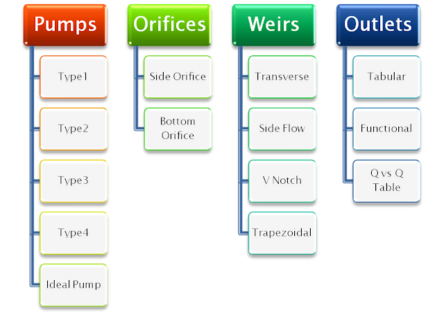
There are ten types of curves in SWMM 5.0.021 in seven categories accessible through the Data Tab and the Attribute Browser – including four types of Pump Curves:


  1. Storage
  2. Diversion
  3. Rating
  4. Tidal
  5. Control
  6. Shape
  7. Pump
    1. Pump1
    2. Pump2
    3. Pump3
    4. Pump4

Figure 1: Curve Types in SWMM 5


Read more…

Types of Nodes and Links in SWMM 5

Subject:  Types of Nodes and Links in SWMM 5


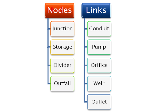
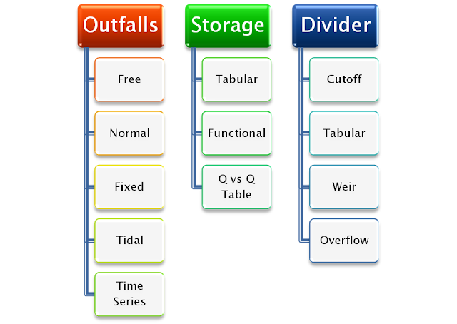
The main objects in a SWMM 5 drainage network are the nodes and links. Nodes are Junctions,  Storages,  Dividers and  Outfalls.  Links are Conduits, Pumps, Orifices, Weirs and Outlets.  There is one type of junction but 5 types of Oufalls, 3 types of Storages and 4 types of Dividers. The dividers can be used in the dynamic wave solution of SWMM 5 but only divide the flow in the kinematic wave solution.


Figure 1.  Node and Link Objects in SWMM 5

Figure 2:  Node Objects in SWMM 5

Read more…

Subject:  SWMM 5.0.021 has 16 Overall Modeling Objects


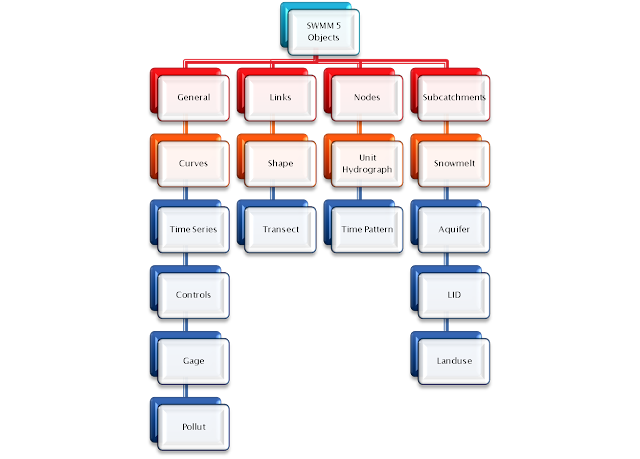
SWMM 5.0.021 has 16 Overall Modeling Objects divided into 4 categories:


1.   General

2.   Subcatchments

3.   Nodes

4.   Links


The objects in the General category can be applied to more than one category. For example, you can simulate pollutants either at a node or at the subcatchment level.


The objects are:

1.           Gage

2.           Links

3.           Shape

4.           Transect

5.           Nodes

6.           Unit Hydrograph

7.           Time Pattern

8.           Subcatchments

9.           Snowmelt

10.                Aquifer

11.                LID

12.                Landuse

13.                Pollut

14.                Curves

15.                Time Series

16.                Controls

Figure 1.  Modeling Objects in SWMM 5.0.021


Read more…

Average Number of Node Iterations

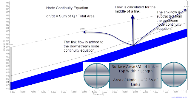
Subject:  SWMM 5 will iterate for the new node depth at each time for a minimum of 2 iterations to a maximum of 8 iterations based on the Node Continuity equation.  If you plot the average number of iterations over time then typically the number of iterations go up as the Inflow increases.  The nodes with the most iterations changes over time as the peak flow moves through the network as shown in this plan view.  The iterations used during the simulation is a function of the node stop tolerance which has a default value of 0.005 feet in SWMM 5.

Read more…

Subject:  How to Import a File from SWMM5 toH20MAP SWMM


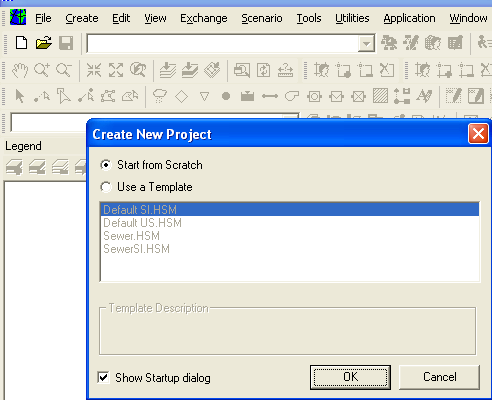
Step 1:  Make a new H2oMAP SWMM Network


Figure 1.  New Network Dialog.


Step 2:  Use the Exchange Tool / Import EPA SWMM 5

Figure 2. Exchange Tool in H20MAP SWMM


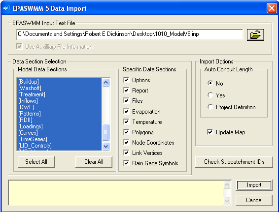
Step 3:  Import your EPA SWMM data file after locating it using the browser.  Click on Import.

Figure 3.  Import Dialog in H2OMAP SWMM.


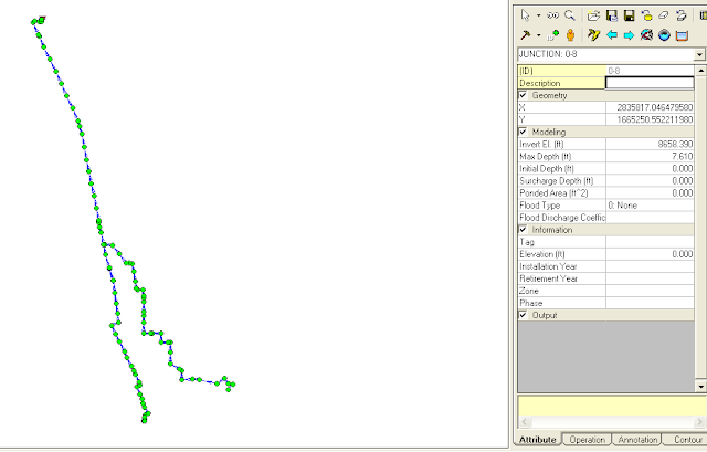
Step 4:  Use the Attribute Browser,  DB Editor and Run Manager to see your data and network after import.

Figure 4.  The imported network in H2oMAP SWMM.


Read more…

Tributary Area to a Node in InfoSWMM

Note:  Tributary Area to a Node in InfoSWMM


Here are the steps you neeed to take to calculate the tributary area of a node in InfoSWMM:


Step 1:  Use the DB Editor to get the total area in your model using the Data Statistics Tool.


Step 2:  Use the Process options in InfoSWMM to ONLY simulate surface runoff and flow routing.


Step 3. Copy the Node name and Total Inflow Volume from the Juntion Summary Output Table to Excel


Step 4:  Find the Total Wet Weather Flow during the simulation from the Wet Weather Inflow Row in the Flow Continuity Table.


Dry Weather Inflow   0.000  0.000

Wet Weather Inflow  0.782   0.255


Step 5. Make a new column in Excel to calculate the tributary area.


The Tributary Area of a Node = Total Inflow Volume / Total Wet Weather Flow * Total Subcatchment Area from Step 1.


You will now have the tributary area for each node.  You can verify this number = the total tributary area at the outfalls should equal the Total Subcatchment Area from Step 1.


Maximum

Maximum

Lateral

Total

Time

of

Lateral

Total

Tributary

Inflow

Inflow

Occurrence

Volume

Inflow

Inflow

Area

Node

Type

CFS

CFS

days

hr:min

10^6 gal

10^6 gal

acres

P001

JUNCTION

5.54

10.86

0

2:27

0.1

0.255

14.74

P005

JUNCTION

2.14

7.42

0

2:26

0.039

0.155

8.96

P009

JUNCTION

5.78

5.78

0

2:25

0.106

0.106

6.13

P011

JUNCTION

0.7

0.7

0

2:34

0.01

0.01

0.58

OUTLET

OUTFALL

0

10.84

0

2:28

0

0.255

14.74


Read more…

MWH Soft Surge Product Line Revs Up Modeling Performance; Breaks Size Barrier for Analyzing All-Pipe Water Networks

Built for Speed and Power, Latest Release Shatters Records and Equips Engineers with Unprecedented Transient Capabilities for Modeling Complex Water Distribution Systems of Any Size

Broomfield, Colorado USA, January 4, 2011

MWH Soft, a leading global innovator of wet infrastructure modeling and simulation software and technologies, today announced the worldwide release of the unlimited link version of its industry-leading surge product line. The breakthrough release brings a new level of software and computational power to the simulation of all-pipe water distribution network models. Available for InfoSurge, H2OSURGE, H2OMAP Surge, and InfoWorks TS, the release is ideal for comprehensive water quality applications that require simulation of very large network models under a wide range of hydraulic transient conditions, from routine operation to emergency states. It has unprecedented power to help users establish proper system-wide coverage, asses their susceptibility to low or negative pressures, estimate potential intrusion volumes and risk to public health, control pressure surges, and minimize the impact of pressure transients should they occur. The enhanced suite reflects MWH Soft’s vanguard position in the water industry and its continuing commitment to delivering pioneering technology for enhancing the safety and reliability of the world’s water supply.

Anticipating and controlling transient response is critical to ensuring the protection, integrity, and effective/efficient operation of water distribution systems. Transient responses can introduce pressures of sufficient magnitude (upsurge) to burst pipes and damage equipment. The resulting repercussions can include extended service outages and loss of property and life. Transient responses can also produce sub-atmospheric pressures (downsurge) that can force contaminated groundwater into the distribution system at a leaky joint, crack or break, leading to grave health consequences when carried out downstream the pipe system. Sustained sub-atmospheric pressures may also lead to cavitation and water column separation, resulting in severe “water hammer” effects as the vapor cavity collapses.

The MWH Soft transient flow simulation technology suite addresses every facet of pressure surge analysis and its role in utility infrastructure management and protection, delivering the highest rate of return in the industry. It provides the engineer-friendly simulation framework water utilities need to identify characteristics that can make their water supply and distribution systems more susceptible to transient pressure events. Users can quickly and efficiently assess the effects of power outages and pump shutdowns, pump startups, valve closures, rapid demand and pump speed changes, and the efficacy of any combination of surge protection devices. The product suite also accurately simulates cavitation and water column separation and evaluates their intensity. Its blazing simulation speed makes transient analysis an easier and more enjoyable task.

Armed with these mission-critical network modeling capabilities, water utilities can more accurately assess their susceptibility to low or negative pressures caused by transient surges, identify vulnerable areas and risks, evaluate and design sound control and mitigation measures, and determine improved operational plans and security upgrades.

“The ability to confidently assess the vulnerability of distribution systems to pressure transients is becoming more critical every day,” said Paul F. Boulos, Ph.D, Hon.D.WRE, F.ASCE, President and Chief Operating Officer of MWH Soft. “Based on close interactions with our customers, we have enhanced our surge product suite to address their most pressing needs for fast and powerful unsteady network simulation capabilities that make it even easier, faster and more cost-effective to apply advanced network simulation technology to manage and operate better, safer water supply and distribution systems.”

Pricing and Availability
The unlimited link version of InfoSurgeH2OSURGEH2OMAP Surge, and InfoWorks TS, is now available worldwide by subscription. For the latest information on the MWH Soft Subscription Program, including availability and purchase requirements, visit www.mwhsoft.com or contact your local MWH Soft Channel Partner.

About MWH Soft
MWH Soft is a leading global provider of wet infrastructure modeling and simulation software and professional solutions designed to meet the technological needs of water/wastewater utilities, government industries, and engineering organizations worldwide. Its clients include the majority of the largest UK, Australasia and North American cities, foremost utilities on all five continents, and ENR top-rated design firms. With unparalleled expertise and offices in North America, Europe, and Asia Pacific, the MWH Soft connected portfolio of best-in-class product lines empower thousands of engineers to competitively plan, manage, design, protect, operate and sustain highly efficient and reliable infrastructure systems, and provide an enduring platform for customer success. For more information, call MWH Soft at +1 626-568-6868, or visit www.mwhsoft.com.

Read more…

How to add a volume variable to SWMM 5

Subject:  How to add a volume variable to SWMM 5


The purpose of this email is to explain how to add another print variable to the DOS version of SWMM 5 so that it can saved in a table in the text output file (after you recompile the modified C code).  The changes have no impact on the SWMM 5 GUI or the SWMM 5 DLL engine.


It is relatively simple five step procedure:


Step 1:  Add a new variable LINK_VOLUME at the end of the link variables in enums.h This is much easier if you just add a report variable that already is part of the link or node structure in objects.h  Your only restriction is that is should be added before the water quality variables.

 // increase by 1 the value of Max  Results in enums.h 
#define MAX_LINK_RESULTS
 7    

enum LinkResultType {
      LINK_FLOW,              // flow rate
      LINK_DEPTH,             // flow depth
      LINK_VELOCITY,          // flow velocity
      LINK_FROUDE,            // Froude number
      LINK_CAPACITY,          // ratio of depth to full depth
      
LINK_VOLUME, // current volume of the conduit - august 2007
      LINK_QUAL};             // concentration of each pollutant
 

Step 2:  Add the report index for LINK_VOLUME to procedure output_open in ouput.c


k = LINK_VOLUME; 
fwrite(&k, sizeof(int), 1, Fout.file);
for (j=0; j<nPolluts; j++)


Step 3: Save the link new volume to the binary output file in procedure link_get_results in link.c.  The new volume of the link has already been saved in the already existing variable newVolume in the Link Structure.


x[LINK_CAPACITY] = (float)c;
x[
LINK_VOLUME]   = (float)Link[j].newVolume;


Step 4. Modify report.c to include the new report variable in procedure report_links


fprintf(Frpt.file, "\n  %11s %8s  %9.3f %9.3f %9.3f %9.1f %9.1f",                          theDate, theTime, LinkResults[LINK_FLOW], LinkResults[LINK_VELOCITY], LinkResults[LINK_DEPTH]  LinkResults[LINK_CAPACITY]* 100.0,
LinkResults[LINK_VOLUME]);

Step 5.  Modify procedure report_LinkHeader in report.c to show the new variable volume:


fprintf(Frpt.file,
"\n                             Flow  Velocity     Depth   Percent   
   Volume");
");
 

Read more…

Rain Barrel LID Fluxes in SWMM 5.0.021


Subject:  Rain Barrel LID Fluxes in SWMM 5.0.021

The fluxes are limited in a Rain Barrel Low Impact Development (LID) control in SWMM 5.  The fluxes only include (Figure 1 and Figure 2):

1.      Total Inflow,
2.      Surface Outflow,
3.      Drain Outflow and
4.      Final Storage

The fluxes are also listed in the LID Performance Summary Table in the output text file.

  ***********************
  LID Performance Summary
  ***********************


  ----------------------------------------------------------------------------------------------------------
                                   Total      Evap     Infil   Surface    Drain      Init.     Final     Pcnt.
                                  Inflow      Loss      Loss   Outflow   Outflow   Storage   Storage     Error
  Subcatchment      LID Control       in        in        in        in        in        in        in
  -----------------------------------------------------------------------------------------------------------
  S1                RainBarrels    110.95      0.00      0.00     62.95     28.15      0.00     23.11    -2.94
Figure 1. Flux Pathways for a Rain Barrel LID

Figure 2. Rain Barrel LID Fluxes


Read more…

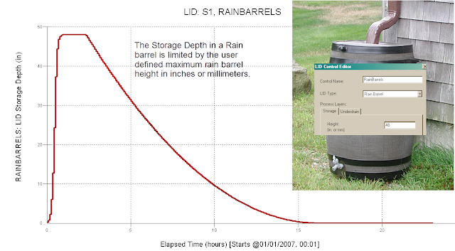
Subject:  Rain Barrel LID Drain Outflow in SWMM 5.0.021

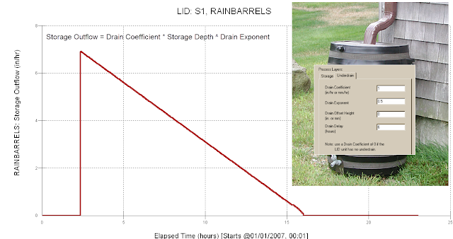
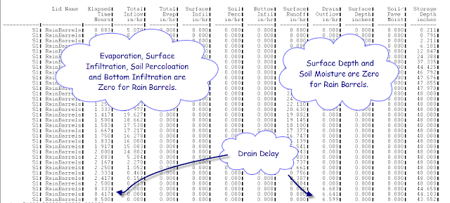
 The drain outflow in a Rain Barrel LID is defined by the user defined drain coefficient and drain exponent and the simulation storage depth  The storage outflow does not occur until it has been dry for at least the drain delay time in hours.
Figure 1.  Storage Outflow or Drain Outflow for a Rain Barrel LID

Figure 2. You can see the effect of the Drain Delay in the output file for LID Simulation.

Read more…

Subject:  What is Hours Above Full Normal Flow in SWMM 5?


The Conduit Surcharge Summary Table in the Report text file or Status Report lists a column of results called “Hours above Full Normal Flow”.  This is the number of hours the flow in the link was above the REFERENCE full flow as calculated by Manning’s equation.  The flow in the link can be above full flow even if the link is not a full depth if the head difference across the link is high enough.  The head difference is the water surface elevation at the upstream end of the link minus the water surface elevation at the downstream end of the link.  The capacity or d/D of the link varies from 0 to 1 with 1 being a full pipe or link.

Figure 1.  Hours above Normal Flow in SWMM 5 Links


Figure 2. Flow versus Full Flow in SWMM 5

Read more…
If you make your tea the old-fashioned way, ending up with a few tea leaves at the bottom of the teacup, and you start stirring the tea, you would expect the leaves to move outward, due to the push of the centrifugal force. Instead the leaves follow a spiral trajectory toward the center the cup. The physical processes that result in this 'tea leaf paradox' are essentially the same as the ones responsible for building point bars in meandering rivers. It turns out that the first scientist to make this connection and analogy was none other than Albert Einstein.
In a paper published in 1926 (English translation here), Einstein first explains how the velocity of the fluid tea flow is smaller at the bottom of the cup than higher up, due to friction at the wall. [The velocity has to decrease to zero at the wall, a constraint called 'no-slip condition' in fluid mechanics.] To Einstein it is obvious that "the result of this will be a circular movement of the liquid" in the vertical plane, with the liquid moving toward the center at the bottom of the cup and outward at the surface (see the figure below). For us, it is probably useful to think things out in a bit more detail.
Einstein's illustration of secondary flow in a teacup
A smaller velocity at the bottom means a reduced centrifugal force as well. But overall, the tea is being pushed toward the sidewalls of the cup, and this results in the water surface being higher at the sidewalls than at the center. The pressure gradient that is created this way is constant throughout the whole water tea column, and overall it balances the centrifugal force (unless you stir so hard that the tea spills over the lips). This means that the centrifugal force wins at the top, creating a velocity component that points outward, but loses at the bottom, creating a so-called secondary flow that is pointing inward. The overall movement of the liquid has a helical pattern; in fact, those components of the velocity that act in a direction perpendicular to the main rotational direction are usually an order of magnitude smaller than the primary flow.

Einstein goes on to suggest that the "same sort of thing happens with a curving stream". He also points out that, even if the river is straight, the strength of the Coriolis force resulting from the rotation of the Earth will be different at the bottom and at the surface, and this induces a helical flow pattern similar to that observed in meandering rivers. [This force and its effects on sedimentation and erosion are much smaller than the 'normal' helical flow in rivers.] In addition, the largest velocities will develop toward the outer bank of the river, where "erosion is necessarily stronger" than on the inner bank.

Secondary flow in a river, the result of reduced centrifugal forces at the bottom

I find the tea-leaf analogy an excellent way to explain the development of river meanders and point bars; just like tea leaves gather in the middle of the cup, sand grains are most likely to be left behind on the inner bank of a river bend. Yet Einstein's paper is usually not mentioned in papers discussing river meandering -- an interesting omission since a reference to Einstein always lends more weight and importance to one's paper (or blog post).

A recent and very interesting exception is a paper published in Sedimentology. It is titled "Fluvial and submarine morphodynamics of laminar and near-laminar flows: a synthesis" and points out how laminar flows can generate a wide range of depositional forms and structures, like channels, ripples, dunes, antidunes, alternate bars, multiple-row bars, meandering and braiding, forms that are often considered unequivocal signs of turbulent flow. As they start discussing meandering rivers and point bars, Lajeunesse et al. suggest that Einstein's teacup is extremely different dynamically from the Mississippi River, yet it can teach us about how point bars form:
A flow in a teacup with a Reynolds number of the order of 102 cannot possibly satisfy Reynolds similarity with the flow in the bend of, for example, the Mississippi River, for which the Reynolds number is of the order of 107. Can teacups then be used to infer river morpho- dynamics?
The answer is affirmative. When dynamical similarity is rigorously satisfied, the physics of the two flows are identical. However, even when dynamical similarity is not satisfied, it is possible for a pair of flows to be simply two different manifestations of the same phenomenon, both of which are described by a shared physical framework. Any given analogy must not be overplayed because the lack of complete dynamic similarity implies that different features of a phenomenon may be manifested with different relative strengths. This shared framework nevertheless allows laminar-flow morphodynamics to shed useful light on turbulent-flow analogues.
Apart from helping understand river meandering, the tea leaf paradox has inspired a gadget that separates red blood cells from blood plasma; and helps getting rid of trub(sediment remaining after fermentation) from beer.

That explains the 'beer' part of the title. And it is time to have one.

References

Einstein, A. (1926). Die Ursache der Meanderbildung der Flusslaufe und des sogenannten Baerschen Gesetzes Die Naturwissenschaften, 14 (11), 223-224 DOI:10.1007/BF01510300

Lajeunesse, E., Malverti, L., Lancien, P., Armstrong, L., Metivier, F., Coleman, S., Smith, C., Davies, T., Cantelli, A., & Parker, G. (2010). Fluvial and submarine morphodynamics of laminar and near-laminar flows: a synthesis Sedimentology, 57 (1), 1-26 DOI: 10.1111/j.1365-3091.2009.01109.x
Source: http://zsylvester.blogspot.com/2010/11/einstein-tea-leaves-meandering-rivers.html
Read more…