All Posts (522)

Sort by

Note:  Storage Maximum Outflow Includes Reverse Flow in SWMM 5

The SWMM 5 text output file has a Storage Volume Summary Table.  The Maximum Outflow from a storage node includes ALL of the outflow from the Storage node including both downstream link flow and reverse flow into the upstream links of the storage node.  You need to look at all of the flow out of a Storage node to find out how the maximum flow was computed during the simulation.

Figure 1.  Storage Volume Summary Table

Figure 2:  Total Flow Out of A Storage Node includes Reverse Flow.
Read more…

Area Types in SWMM 5 for Links with Offsets


Subject:  Area Types in SWMM 5 for Links with Offsets

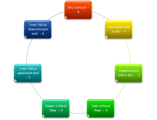
 There are six types of link flow in SWMM 5:

1.   Dry Conduit at both Ends
2.   Upstream End is Dry
3.   Downstream End is Dry
4.   Subcritical Flow
5.   SuperCritical Flow
6.   Free Fall at Upstream End
7.   Free Fall at Downstream End
Figure 1.  Six types of Link Area Allocation

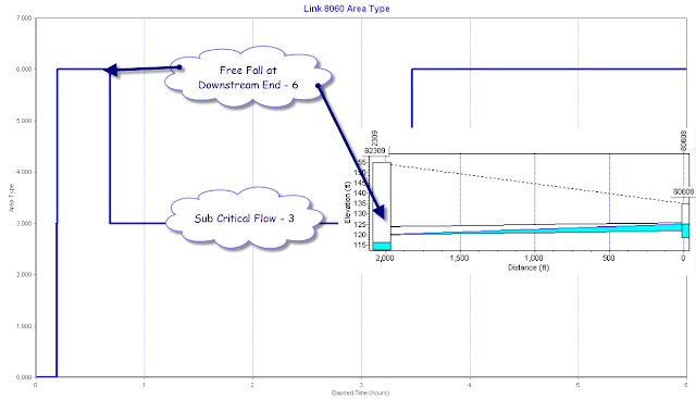
Figure 2.  Example Link Area Type in SWMM 5
Read more…

Force Main Friction Loss in SWMM 5


Subject:  Force Main Friction Loss in SWMM 5

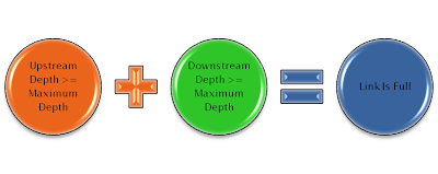
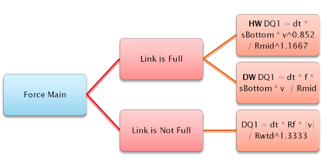
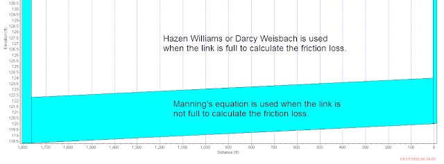
You can model Force Mains in SWMM 5 using either Darcy Weisbach or Hazen Williams as the full pipe friction loss method (see Figure 1 for the internal defintion of full flow).   No matter which method you use for full flow the  program will use Manning’s equation to calculate the loss in the link when the link is not full (see Figure 2 for the equations used for calculating the friction loss – variable dq1 in SWMM 5).   The regions for the different friction loss equations are shown in Figure 3.
Figure 1.  How the full pipe condition is defined in SWMM 5


Figure 2:  Friction equations used in SWMM 5 for a Force Main.


Figure 3:  Regions of Friction loss equations in SWMM 5.


Read more…

Lightning Captured by X-Ray Camera


Lightning.
Scientists triggered lightning using rockets (pictured).

Photograph courtesy Dustin Hill

Richard A. Lovett in San Francisco

for National Geographic News

Published December 23, 2010

http://news.nationalgeographic.com/news/2010/12/101223-lightning-x-rays-camera-science-technology/

The first x-ray images of a lightning strike have been captured by a, well, lightning-fast camera, scientists say. The pictures suggest a lightning bolt carries all its x-ray radiation in its tip. (Get lightning facts.)

During recent thunderstorms in Camp Blanding, Florida, the camera's electronic shutter "froze" a lightning bolt—artificially triggered by rockets and wires—as it sped toward the ground at one-sixth the speed of light.

"Something moving this fast would go from the Earth to the moon in less than ten seconds," said Joseph Dwyer, a lightning researcher at the Florida Institute of Technology in Melbourne.

Scientists have known for several years that lightning emits radiation, said Dwyer, who revealed the photos at an annual meeting of the American Geophysical Union in San Francisco earlier this month.

But until now scientists didn't have the technology to take x-ray images quickly enough to see where the radiation comes from, he said.

(Read "New Lightning Type Found Over Volcano?")

Lightning Imaged by 1,500-Pound Camera

Making a camera capable of taking such quick images was an achievement in and of itself, Dwyer emphasized.

"You can't just go buy a camera and point it at lightning," he said. "We had to make it."

The resulting 1,500-pound (680-kilogram) camera—created by Dwyer's graduate student Meagan Schaal—consists of an x-ray detector housed in a box about the size and shape of a refrigerator. The box is lined with lead to shield the x-ray detector from stray radiation.

X-rays enter the box through a small hole that in turn focuses them, like an old-fashioned pinhole camera.

Speedy Trade-Off: Less Data Space

Because lightning moves blindingly fast, the camera was required to take ten million images per second. (Interactive: Make your own lightning strike.)

One challenge in taking such fast pictures is storing the data. To do so, the x-ray detector had to take pictures at a relatively low resolution of 30 pixels, which produced images on a crude, hexagonal grid—as shown in the chart below.


A chart shows x-ray observations of a lightning discharge.

Diagram courtesy Joseph Dwyer

Even so, the resolution was sharp enough to reveal a bright ball of x-rays at the head of the bolt, with almost no lingering radiation along the bolt's trail.

"Almost all the x-rays are from the tip," Dwyer said. "We see the x-ray source descending with the lightning at up to one-sixth the speed of light."

Triggered Lightning Effective

The lightning bolts were triggered by launching small rockets into the thunderstorms. (See "Volcanic Lightning Sparked by 'Dirty Thunderstorms,' Study Finds.")

The rockets trailed wires behind them to direct the lightning through the camera's field of view.

Artificially triggering the lightning strike likely didn't alter the natural workings of the thunderstorm, Dwyer noted.

And, he said, "the advantage of triggered lightning is that we can repeat it."

Read more…

Capacity Limited Links in SWMM 5

Subject: Capacity Limited Links in SWMM 5


The table in the text report file of SWMM 5 called “Conduit Surcharge Summary” has a column entitled “Hours Capacity Limited” Here is how a link is defined as Capacity Limited in SWMM 5. Two factors have to be present:

1. The upstream end of the link has to be full and

2. The HGL Slope has to be greater than the Slope of the Link


Read more…

What is the Area of a Node in SWMM 5?

Subject: What is the Area of a Node in SWMM 5?


The minimum area of a node is the default area of the node, which is the user defined minimum surface area or 12.566 square feet if the user does not define the surface area of the node. The surface area of a node is usually the half of the surface area of all of the connecting conduits but if the link is dry then the sum of all of the surface areas may be less than the default surface area. If you look at a scatter plot of the area versus the depth then you will see that it always has the minimum surface area.


Read more…

What is Node Convergence in SWMM 5?

Subject:  What is Node Convergence in SWMM 5?

 If a link has converged within two iterations then the hydraulic computations will be bypassed for the link in new iterations.  A link is deemed converged if BOTH the upstream and downstream node depth has converged between successive iterations as long as two iterations have occurred during the time step.  The nodes are considered converged if the depths between successive iterations is less than the stop tolerance of the program (the default stop tolerance is 0.005 inches).  The new node depths are ALWAYS computed for each iteration but the links connected to the converged nodes may bypass computations and save on simulation time.  Note:  If the nodes ever become non converged after 2 iterations then the link flows will be computed.


Read more…

What is Link Bypass in SWMM 5?

Subject:  What is Link Bypass in SWMM 5?


If a link has converged within two iterations then the hydraulic computations will be bypassed for new iterations.  A link is deemed converged if BOTH the upstream and downstream nodes depth has converged between successive iterations as long as two iterations have occurred during the time step.  This is simulation savings step as it my eliminate up to 75 percent of the computational time in a SWMM 5 simulation.  The image below shows that for some links the flow in the link is converged within 2 iterations whereas for others it may take 3 or 4 iterations.  Overall, 37 percent of the link computations are bypassed during the simulation of this particular hydraulic network.


Read more…

Poisson Distribution

Poisson Distribution

06 JUN 2007   by David Harper, CFA, FRM, CIPM  Source http://www.bionicturtle.com/how-to/article/poisson_distribution/

le_painter

2007 FRM Learning outcome 2.7: Calculate the expected value and variance of the Poisson distribution.

What is the Poisson used for?

The Poisson is related to the binomial distribution. In the binomial distribution, we conduct Bernoulli trials. That is, trials with two outcomes; e.g., success/failure, up/down, incoming service center call/no call. We use the Poisson to characterize variables over time (or over space). For example,

  • http://www.bionicturtle.com/assets/images/article-li.gif); background-attachment: initial; background-origin: initial; background-clip: initial; background-color: initial; background-position: 4px 6px; background-repeat: no-repeat no-repeat; border: 0px initial initial;">How many operational errors are expected per day/month/year?
  • http://www.bionicturtle.com/assets/images/article-li.gif); background-attachment: initial; background-origin: initial; background-clip: initial; background-color: initial; background-position: 4px 6px; background-repeat: no-repeat no-repeat; border: 0px initial initial;">How many typos are expected per page?


What is the pdf?

Hopefully FRM candidates know by now that pdf refers to probability density function (pdf). Note the pdf is also sometimes called the probability mass function. We can describe a distribution by its local density (what is probability that random variable X will equal value x?) or its cumulative distribution function (what is the probability that random variable X will be less than or equal tovalue x?). Further, distributions can be discrete or continuous (e.g., the normal).

The Poisson is discrete:

lambda1


Lambda is the key parameter. Lambda is both the mean (expected value) and the variance! What is the expected value of an an event over time? It is simply the rate of occurrence (r) multiplied by time (t). So we could expand the Poisson pdf out to this:

lambda2


So, the things to remember are:

  • http://www.bionicturtle.com/assets/images/article-li.gif); background-attachment: initial; background-origin: initial; background-clip: initial; background-color: initial; background-position: 4px 6px; background-repeat: no-repeat no-repeat; border: 0px initial initial;">Poisson is discrete
  • http://www.bionicturtle.com/assets/images/article-li.gif); background-attachment: initial; background-origin: initial; background-clip: initial; background-color: initial; background-position: 4px 6px; background-repeat: no-repeat no-repeat; border: 0px initial initial;">The expected value is the mean (rate x time) which is called lambda. Lambda is both the mean and the variance

An example

Let's say we observe our company commits a certain sort of operational error (e.g., bad invoice) ninety times per month. How many errors should we expect in a single day. The mean is (90)(1/30) = 3. So, lambda is three and three is the expected number of errors per day. The Poisson distribution is given below in the EditGrid spreadsheet. Note that I used both the built-in formula and the actual function. You can open your own read/write copy here.

Risk (FRM) >

Read more…

Time Step Critical Elements in SWMM 5

Subject:  Time Step Critical Elements in SWMM 5

The time step critical elements in the SWMM 5 report text output file tells you which elements were controlling the time step during the simulation.  If no element was controlling the time step then the program will just use the maximum time step.  For example, if the maximum time step was 10 seconds and the average time step was 9.8 then only a few time steps were set by a link or node that needed a smaller than maximum time step (Figure 1).  If the maximum time step for the same simulation was 30 seconds then many links and nodes will set the time step (Figure 2).


Figure 1.  Most of the time the simulation used the maximum time step of 10 seconds so only a few links were time step critical.

Figure 2.  Most of the time the simulation used less than the maximum time step of 30 seconds so many links were time step critical.

Read more…

Pump Power Usage in SWMM 5

Subject:  Pump Power Usage in SWMM 5


 The pumping summary table (Figure 1) includes a column that tells the user how much power was consumed by the pump in kilowatts by the head loss or head gain of the water flowing through the pump. The power usage equations are shown in Figure 2.


 Figure 1.  Pump Summary Table in SWMM 5.0.021


Figure 2.  Pump Power Equations in SWMM  in which dt is the time step.


Read more…

Shanghai Makes MWH Soft’s InfoWorks WS Solution Its Water Distribution Modeling Platform


Largest City in World’s Most Populous Country Looks to Advanced MWH Soft Technology
to Improve Drinking Water Operations and Planning


Broomfield, Colorado USA, July 14, 2010 — MWH Soft, a leading global innovator of wet infrastructure modeling and simulation software and technologies, today announced that Shanghai Municipal Water Supply Dispatching and Monitoring Centre (SH MWSDMC) has chosen InfoWorks WS as its preferred modeling platform. The selection further substantiates MWH Soft’s global leadership position in geospatial wet infrastructure modeling and management.


Serving over seventeen million people, SH MWSDMC deals with enormous challenges in managing the delivery of adequate water supply. The Centre manages the GIS and SCADA system for the entire Shanghai water network and oversees the transfer of water between four regional water companies.


“We chose the InfoWorks WS solution for its ability to model large networks with speed and efficiency,” said the Centre’s Vice Director Mr. Zhao Pingwei. “I’ve been familiar with InfoWorks WS for many years, and found it to be the best fit for our needs.”

Around the world, high quality all-mains InfoWorks WS models enable utilities to make informed planning and management decisions with confidence by giving them an accurate view of their water distribution systems’ performance. This information — including water quality, supply, demand and infrastructure problems and investigations of remedial measures — allows them to provide a sustainable supply of high quality water at an acceptable pressure and flow rate to commercial, industrial and domestic users while minimizing loss through leakage. As part of the advanced MWH Soft workgroup modeling management platform, InfoWorks WS is built to handle large models and allow robust multi-user collaboration.

The InfoWorks platform offers a complete solution: all the needed tools, simulations and data integration are included in a single application. Building models is simplified by an intuitive user interface and robust GIS integration that maximizes productivity, reduces likelihood of errors and enables users to move swiftly between modeling functions.


InfoWorks WS presents results and reports in a fully interactive interface, allowing users to open any number of maps, tables, profiles and graphs at the same time. Reporting options include maps (with color coding and symbology), contours, customized labeling, tables, graphs, profiles, 3D views, animations, SQL selections, Google Earth exports, stored views, and custom MS Excel reports.


InfoWorks WS has proven to be the hydraulic modeling package of choice for China’s wet infrastructure community,” said MWH Soft Asia Pacific Business Development Manager Justin Hanson. “The selection by Shanghai further confirms that utilities which invest in MWH Soft technology gain a superior technological advantage that will lead to measurable improvements in productivity, system performance, and customer satisfaction.”

Read more…

MWH Soft FloodWorks Successfully Predicts Flash Flooding in Egypt

Advanced Flood Forecasting Software Helps Save Lives and Minimize Damages


Broomfield, Colorado USA, March 17, 2010 — MWH Soft, a leading global innovator of wet infrastructure modeling and simulation software and technologies, today announced the successful implementation of its FloodWorks software in a 3900 mi2 (10,000 km2) pilot area around Nuweiba, Egypt. The system was used to successfully predict flooding in the region in February 2010, the worst flash flooding event in Egypt since 1994. The implementation is the latest expression of MWH Soft’s industry-leading commitment to creating groundbreaking software tools for real time hydraulic and hydrologic modeling.

Nuweiba, on the southeastern portion of the Sinai Peninsula, is located on a floodplain sandwiched between the Gulf of Aquaba and the Sinai Mountains. Although the peninsula suffers from frequent water shortages, it is subject to flash floods that result in loss of life, hamper regional development, and greatly contribute to soil erosion and pollution. The February 2010 flooding resulted in significant damage and seven deaths. In the pilot area running MWH Soft FloodWorks, no casualties were reported.

FloodWorks is a modular software package for real-time simulation and forecasting of extreme hydrological and hydraulic conditions within river basins, drainage systems and coastal zones. Linking real-time hydrological and meteorological time-series data sources with detailed and accurate hydraulic models, it forecasts water level, flood depth and sea state for the hours or days ahead. Designed for operational use in the control room, FloodWorks is particularly suited to real time flood forecasting, warning and management of river catchments and coastal areas. Critical to the program is its ability to aggregate multiple sources of dynamic input data and automatically validate them in real time. This capability, combined with the flexibility to work with InfoWorks RS, InfoWorks CS, InfoWorks ICM, InfoSWMM, H2OMAP SWMM, and other non-MWH Soft hydrologic and hydraulic simulation models, makes FloodWorks both easy to implement and highly accurate.

By enabling managers and engineers to carry out fast, accurate simulation of the future behavior of river and channel systems, FloodWorks supports the mobilization of emergency responses and the issuance of public flood warnings. It can also be used to support reservoir and dam operations, predict low flow episodes, and generate real-time water quality predictions and warnings.

“MWH Soft is committed to providing the best wet infrastructure technology for building a better world,” said Andrew Brown, the company’s EMEA Regional Manager. “Real time modeling and forecasting involves some of our most advanced technology. It has the potential to not only dramatically improve emergency response to flooding events, but save lives.

“For computer-modeled flood forecasting to be useful, it must be both extremely accurate and very fast. As shown during the Egypt flooding, FloodWorks clearly meets these criteria. We look forward to offering the FloodWorks product line to governments throughout the world seeking better ways to alert their flood managers, citizens, and first responders; mobilize temporary flood control devices; and most importantly, prevent loss of life.”

About MWH Soft
MWH Soft is a leading global provider of wet infrastructure modeling and simulation software and professional solutions designed to meet the technological needs of water/wastewater utilities, government industries, and engineering organizations worldwide. Its clients include the majority of the largest North American cities, foremost utilities on all five continents, and ENR top-rated design firms. With unparalleled expertise and offices in North America, Europe, and Asia Pacific, the MWH Soft connected portfolio of best-in-class product lines empower thousands of engineers to competitively plan, manage, design, protect, operate and sustain highly efficient and reliable infrastructure systems, and provide an enduring platform for customer success. For more information, call MWH Soft at + 1 626-568-6868, or visit www.mwhsoft.com.

Read more…

Warmer Planet Temperatures Could Cause Longer-Lasting Weather Patterns

ScienceDaily (Feb. 21, 2010) — Whether it's never-ending heat waves or winter storms, atmospheric blocking can have a significant impact on local agriculture, business and the environment. Although these stagnant weather patterns are often difficult to predict, University of Missouri researchers are now studying whether increasing planet temperatures and carbon dioxide levels could lead to atmospheric blocking and when this blocking might occur, leading to more accurate forecasts.


"In this research, we're trying to see if increased carbon dioxide in the atmosphere and the resulting atmospheric warming will affect the onset and duration of future blocking events," said Tony Lupo, professor and chair of the atmospheric science department at the MU College of Agriculture, Food and Natural Resources. "We're hoping that the research will add cues that could help fellow forecasters better predict blocking and warn people in cases of long-lasting, severe weather."

Atmospheric blocking occurs between 20-40 times each year and usually lasts between 8-11 days, Lupo said. Although they are one of the rarest weather events, blocking can trigger dangerous conditions, such as a 2003 European heat wave that caused 40,000 deaths. Blocking usually results when a powerful, high-pressure area gets stuck in one place and, because they cover a large area, fronts behind them are blocked. Lupo believes that heat sources, such as radiation, condensation, and surface heating and cooling, have a significant role in a blocking's onset and duration. Therefore, planetary warming could increase the frequency and impact of atmospheric blocking.

"It is anticipated that in a warmer world, blocking events will be more numerous, weaker and longer-lived," Lupo said. "This could result in an environment with more storms. We also anticipate the variability of weather patterns will change dramatically over some parts of the world, such as North America, Europe and Asia, but not in others."

Lupo, in collaboration with Russian researchers from the Russian Academy of Sciences, will simulate atmospheric blocking using computer models that mirror known blocking events, then introduce differing carbon dioxide environments into the models to study how the dynamics of blocking events are changed by increased atmospheric temperatures. The project is funded by the US Civilian Research and Development Foundation -- one of only 16 grants awarded by the group this year. He is partnering with Russian meteorologists whose research is being supported by the Russian Federation for Basic Research.

Lupo's research has been published in several journals, including the Journal of Climate and Climate Dynamics. He anticipates that final results of the current study will be available in 2011.

Story Source:
Adapted from materials provided by University of Missouri-Columbia, via EurekAlert!, a service of AAAS.

Read more…

SWMM 5 Pump Curve Head/Flow Curves (1)

Subject: The Pump flow is based on the lookup table you enter for the pump (Figure 1). At each iteration during each time step of the solution SWMM 5 will look up the flow for the pump based on the current control variable across the pump. The control variable for the pump can be one of four variables:

1.The volume of the upstream wet well,

2.The depth of water at the upstream node or inlet node without interpolation between data points,

3.The downstream water surface elevation across the pump minus the upstream water surface elevation, and

4.The depth of water at the upstream node or inlet node with interpolation between data points.

The pump summary table in the rpt file will tell you how often the pump was used, the maximum flow, the average flow, the total volume of the pump, the power usage and the percent of the time off the entered pump curve. You can also plot the pump flow versus the inlet depth to see how often the pump was off the pump curve (Figure 2).

Figure 1: Plot of Head and Flow for Pump PUMP1@82309e-15009e over time along with the input and output table for the pump.

Figure 2: Plot of Head versus Flow for Pump PUMP1@82309e-15009e

Read more…

Subject: Reserve Capacity and Flow in a Link

The Reserve flow and Reserve Capacity are modeling guidelines and do not actually influence the computed flows in a link. If you have a positive Reserve flow or capacity then you MAY get more flow in the link based on the current flow being less than the Qfull for the link but not if the link is under surcharge, has backwater conditions or has large entrance and exit losses. You cannot always assume that because the Reserve flow is positive the link can handle more upstream flow.

Here are few graphs that show the relationship between Qfull, the actual Q in the link and the Reserve Flow or Reserve Capacity. The Qfull is a reference flow and is not used during the computation in InfoSWMM and SWMM5.

Condition 1: Positive Reserve Flow – the flow is always less than Qfull and the Reserve flow and Reserve Capacity are Positive.

Condition 2: Negative Reserve Flow – the flow is sometimes greater than Qfull and the Reserve flow and Reserve Capacity are negative when this occurs.

Reserve Capacity – the Reserve in the link * the current link volume.


Read more…

Explicit Iteration Hydraulic Computation and Implicit Time Step Hydraulic Computations in SWMM 5


The dynamic wave solution in SWMM 5 and InfoSWMM uses an interlocking explicit iteration in an overall time step implicit calculation of the node depths and link flows. The node depths and links flows are computed based on the last iteration values for 2 to 8 iterations. It explicitly calculates the node depths and link flows at each iteration based on the last iteration value but uses an underrelaxation or Gauss-Seidel method averaging to compute the final new iteration values. The underrelaxation method averages the last iteration value and the current iteration estimate to calculate the final iteration node depth and links flow.


At each time step this is the sequence of computations:


1. The time step is based on the Courant–Friedrichs–Lewy (CFL) condition for the most restrictive link (the CFL condition is based on the link length, current depth and current velocity),

2.Link flows and node depths are calculated at the 1st iteration based on the last time steps flows and depths,

3. The new iterations link flow and node depths are calculated by averaging the node depths and link flows found in step 2 with the original iteration node depths and link flows,

4. The iteration process continues for at least 2 iterations for all nodes and links,

5. The iteration process may stop after 2 iterations for those links in which the upstream and downstream node depths have converged,

6. The upstream or downstream node is considered converged when the absolute depth difference between iterations is less than 0.005 feet,

7. The maximum number of iterations for all nodes and links is set to 8.

8. Once the number of iterations has reached 8 or all nodes and links are converged the time step calculations are considered finished and the program moves on to a new time step.

9. The image shown below shows how the node continuity equation is solved for each iteration but the link combined continuity and momentum equation is calculated for either 2, 3 or 8 iterations depending on the upstream and downstream node convergence of the link.


Read more…

Export from WeatherUnderground to InfoSWMM

Note: Export from WeatherUnderground using the CSV File Export Option to InfoSWMM


Weather Underground is a site that provides excellent local weather information in the form of graphs, tables and csv files. You can use the data very easily in InfoSWMM by copying from Excel to a time series in InfoSWMM. Here is the rainfall for a storm event in Tampa, Florida in September 11, 2010

Step 1: Export from WeatherUnderground using the CSV File Export Option

Step 2: The data imported from the csv file to Excel and after the text to columns tool is used looks like this in Excel. The data is now ready to be imported into InfoSWMM after the time column is adjusted to fall on even 5 minute intervals. In Excel you can use the formula @ROUND((B2)/"0:05:00",0)*"0:05:00" to round all of the time values to 5 minutes. If you do not do this step then you will have problems in InfoSWMM due to the rainfall interval not being equal to the defined raingage interval.


Step 3: You will need to format the new rounded time as a time format for import into a InfoSWMM time series. The time series is created in the operation tab of the attribute browser.


Step 4: Open up and make a new time series in InfoSWMM.


Step 5: Copy and then paste the date, rounded time column and rainfall column into the InfoSWMM time series columns.


Step 6: Make a raingage in the DB Table in InfoSWMM that will use the time series you just made. In the case of the Weather Underground data we will use inches, intensity, a rainfall interval of 5 minutes, time series and the name of the time series. SCF should be 1 for Snow conversion and do not need to include a Filename or Station name as we are not using an external file.


Read more…

RDII Import into InfoSWMM

Note: InfoSWMM and H2OMAP SWMM can import any version of the RDII Unit Hydrograph data from SWMM 5.0.001 to SWMM 5.0.021 using the Import manager command. The difference is that SWMM 5.0.013 and earlier versions had less initial abstraction data and versions after SWMM 5.0.014 had more initial abstraction data. However, the Import Manager detects the version and imports the data correctly. SWMM 5.0.013 stored 9 RTK and 3 Initial Abstraction parameters and later versions 9 RTK and 9 Initial Abstraction parameters. InfoSWMM will import any format into the current version of InfoSWMM or H20MAP SWMM, which is based on SWMM 5.0.018 but will soon be based on SWMM 5.0.021.

SWMM 5.0.001 to 5.0.013 RDII UH Data

SWMM 5.0.014 to 5.0.021 RDII UH Data


InfoSWMM and H2oMAP SWMM will have 9 RTK and 9 Initial Abstraction Parameters.

Read more…